Daily-Log Vishwa

4/29/2024 Deep Vibe

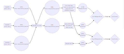
Data Collection: There are three DeepVibe sensor nodes, each labeled as "sensor node 1", "sensor node 2", and "sensor node 3". These nodes are collecting sensor measurement(s) and sending payloads to the DeepVibe root node via a WiFi connection. This implies a distributed sensor network where each node is likely to be placed at different monitoring points.

The DeepVibe root node acts as a central aggregator or hub, collecting the data payloads from each sensor node. This root node is equipped with a USB interface, suggesting it can be connected to a computer or server for data processing or to an S3 sandwich device which is capable of further transmitting data.

1. Data Processing:

   A Linux Socket App receives sensor measurements via USB from the root node. This application sends raw measurements and processes the latest Fast Fourier Transform (FFT) to analyze the frequency components of the sensor data. Notably, the CEEMDAN algorithm is disabled, possibly for efficiency or due to resource constraints.

   • An S3 sandwich device also receives data from the root node via USB. It appears to function as a bridge by taking this data and sending it over RESTful HTTP requests, potentially to a server or cloud service.

2. Data Storage: The processed data from the Linux Socket App and the raw data from the S3 sandwich are sent to both a local and a cloud TDEngine service. TDEngine is likely used for its time-series database capabilities, which are suitable for sensor data.

3. Visualization and Monitoring: Both local and cloud TDEngine services are connected to instances of Grafana. The "Plugin" notation indicates custom plugins or configurations for Grafana, potentially for specific visualization requirements.

4. Data Migration: Mentioned in the text is a migration from TDEngine to TimescaleDB, which is a scalable SQL database designed for time-series data. will involve changes to the linux_socket_app and deepvibe-dsp-c components.

Comments:

Review S3 sandwich(one s3 replaces the raspberry pi in the raspberry pi-S3 combo )

Local grafana local DB missing in architecture

Ask jacob (move repos to deepvibe folder)

Drf (Django Rest framework YTvideo)

Django REST Framework (DRF) is a powerful toolkit for building Web APIs in Django

Here are some key features of Django REST Framework:

1. Serialization: DRF provides a powerful serialization engine that allows you to convert complex data types, such as Django model instances, into native Python data types that can then be easily rendered into JSON, XML, or other content types.

2. Views: DRF includes a set of generic views that can be used to quickly build common API patterns, such as CRUD (Create, Retrieve, Update, Delete) operations.

3. Authentication: DRF includes session authentication, token authentication, OAuth, and JWT authentication. This makes it easy to secure your API endpoints with different authentication mechanisms.

Comments :

Epoch : 1970

Change table names

Change api calls

4/30/2024

Understanding FFT and Liquid DSP

Used for processing of signal data

The FFT algorithm reduces the computational complexity of computing the DFT from 𝑂(N^2) to O(NlogN), where N is the number of data points. This efficiency makes it practical to perform Fourier analysis on large datasets in real-time or near real-time applications.

DSP involves manipulating signals to enhance them or to extract meaningful information. It can involve operations such as filtering, compression, feature extraction, and more.

How to listen on serial port with C using CRTSCTS

What is CRTSCTS?

RS232 standard. It makes use of two further pins on the RS232 connector, RTS (Request to Send) and CTS (Clear to Send). These two lines allow the receiver and the transmitter to alert each other to their state.

configuring a serial port in a Linux environment to read from an Arduino device without causing it to reset upon connection.?

trying to manage the Data Terminal Ready (DTR) signal such that it doesn't reset the Arduino when your computer restarts or when the connection is re-established. ?

also trying to enable hardware flow control (CRTSCTS) correctly in my C program.?

Comments

• D-oxygen c documentation (ask jacob & melisa)
• Timescale Db repo (understand / curl command usage? Better alternatives)
• curl command usage : Downloading files from web servers
• Uploading files to servers
• Making HTTP requests and receiving responses

Doxygen calls :

@file The file name must be present in the file header for inclusion into the documentation generation process

@param Parameter documentation for functions

@page Markdown page name

@mainpage Main markdown page for the project

@tableofcontents Generates “table of contents” for the markdown page**

• The @brief tag gives a concise description of what the function does.
• The @param tags describe the purpose of each parameter.
• The @note and @warning tags provide additional contextual information**

Time scale DB:

Functions:

*drf_write_callback: callback function to handle the response from the REST API.*

*print_the_drf_payload: function to print the payload data*

*post_to_DRF: function to send POST requests to the REST API with a payload.*

*post_acc_history_to_DRF_test: function to post accelerometer data to the REST API.*

Changes : Removed assignment operators for macros

Usage : const char *accel_hist_end_point = API_ENDPOINTS[ACCEL_HIST] then we will hit the

localhost:8000/api/accelerometer-history/

int main() {

const char *accel_hist_end_point = API_ENDPOINTS[ACCEL_HIST];

const char *latest_acceleration_end_point = API_ENDPOINTS[LATEST_ACCEL];

const char *bme280_hist_end_point = API_ENDPOINTS[BME280_HIST];

const char *ds18b20_hist_end_point = API_ENDPOINTS[DS18B20_HIST];

const char *analog_sensor_hist_end_point = API_ENDPOINTS[ANALOG_HISTORY];

const char *latest_fft_end_point = API_ENDPOINTS[LATEST_FFT];

const char *latest_ceemdan_end_point = API_ENDPOINTS[LATEST_CEEMDAN];

const char *node_details_end_point = API_ENDPOINTS[NODE_DETAILS]

Checked : tty.ccflag &= ~CRTSCTS (looking for work arounds)?_

Add manually # define CRTSCTS 020000000000

Fixed : added #include <asm-generic/termbits.h>

explanation : The <asm-generic/termbits.h> header is part of the Linux kernel headers and provides more extended capabilities like CRTSCTS

Comments : sphinx, nbdev, pydocs (ask jacob)

Check markdown!

Sinus & Skull Base Surgery Virtual Surgical Planning Software

• Surgeon inputted planning data could also be used to help develop artificial intelligence algorithms

efforts could be made to establish a CPT code for reimbursement for planning work performed during surgery(CPT code)? : Current Procedural Terminology (CPT) codes are numbers that identify the services and supplies a patient receives from a healthcare provider.

INPUT : Using radiological inputs including DICOM files from pre-operatively obtained computed tomography (CT) and magnetic resonance imaging (MRI), create an interactive 3D model. This model should be modifiable and allow surgeons to remove tissue,

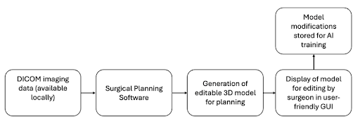
Preliminary approach :

Import and Initial Processing

Libraries like pydicom for Python, would be ideal for reading, modifying, and writing DICOM

https://github.com/pydicom/pydicom

https://pydicom.github.io/

Data Merging and 3D Modeling

Technologies: libraries like VTK or ITK()Insight Segmentation and Registration Toolkit, an open-source library that provides software tools for image analysis (computer graphics, modeling, image processing) for processing and merging CT and MRI data. They create meshes and structures.

Surgical Planning and Simulation

Create modules for simulating surgeries, like tissue removal, using physics engines integrated within Unity3D and unreal engine

Implementation :

https://www.unrealengine.com/en-US/spotlights/helping-brain-surgeons-practice-with-real-time-simulation

https://www.unrealengine.com/en-US/spotlights/precision-os-delivers-accredited-curriculum-for-orthopedic-surgical-training-in-vr

https://scikit-image.org/docs/stable/auto_examples/edges/plot_marching_cubes.html

5/1/2024

Sinus & Skull Base Surgery Virtual Surgical Planning Software

3D Volume Rendering:

The CT scan produces a series of 2D slices showing the internal anatomy.

A CT scan shows detailed images of the bones, muscles, fat, and organs ... axial, images (often called slices) of the body. ... internal organs and other ...thumbs_up_down

Software can process these slices and assign colors or densities based on the X-ray attenuation of different tissues.

By stacking these colored slices together, a 3D volume is created, allowing visualization of organs, bones, and other structures.

Volume Rendering: By stacking multiple axial slices together, a volume dataset can be created. Volume rendering techniques can then be applied to this dataset to generate 3D images. These images provide a more comprehensive view of the internal structures and can be manipulated to highlight specific tissues or organs

Segmentation:

Software can identify and isolate specific structures in the CT scan based on their density or other characteristics.

This segmentation process creates separate 3D models for bones, muscles, blood vessels, or other features of interest.

These models can then be manipulated, analyzed, or used in 3D printing applications.

Surface Reconstruction:

This method focuses on creating a 3D surface representation of the scanned object.

Algorithms analyze the CT data to identify the boundaries between different tissues.

The resulting surface model can be useful for visualizing the external shape of bones, organs, or other structures

Comments :

Talk to jake abt (workon) particular way of virtual environment/ jupyter notebook , conda

2D to 3D medical image colorization.

Modality Conversion: The first method involves converting 3D MRI data into a "photographic volume" using Generative Adversarial Networks (GANs)

Style Transfer: Once the MRI data is converted, selected slices are stylized using neural style transfer techniques, leveraging a 2D style exemplar image.

Volume Colorization: colorizing the entire volume based on the stylized slices. involves advanced optimization techniques

Comments :

Understand

Initial exploration of CT data using 3d slicer

(segmentation) (discuss limitations)

Reflection of my journey

Visual studio 2022 license (ask jake)

5/2/2024

DICOM serves as the standard format for radiology reports, with files commonly using the extension “.dcm”

Installed wsl

notes on cppcheck(UC cybersecurity)

afternoon -Explore colab (terminal) (tmux)

( https://general.gqc.com/dev/Linux/tmux

Some more specific details of why we started using tmux:

https://general.gqc.com/dev/Linux/wsl/setup

In this second one, you can skip to the tmux section and read through it. )

Switch to deepvibe, timescaleDB, DRF repo

Created a Simple Image Processing App with MONAI Deploy App SDK

Tested a simple image processing app with monai

SobelOperator: Applies a Sobel edge detector, the image data (as a Numpy array) is set to the output

MedianOperator: Applies a Median filter for noise reduction.

GaussianOperator: Applies a Gaussian filter for smoothening.

Compiled dicomm_series_to_image_app (no visible output, fixed dependency and package import issues)

https://github.com/eidelen/DicomToMesh (share this to sudhir and get feedback)

Tmux

tmux is a terminal multiplexer. It lets you switch easily between several programs in one terminal,

GQC uses tmux to ensure processes running in Linux, such as long jobs on MSI Server

Open a tmux session with "tmux".

We can start the long-running task on the MSI.

Then press "Ctrl + b d" to detach from the session.

You can then close the window.

You can reattach to the session with "tmux a"

Switching to deepvibe

Deep_Vibe Server

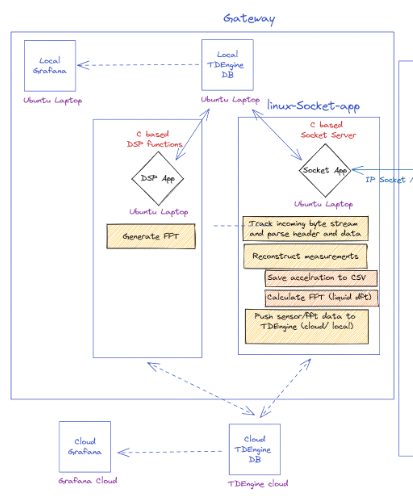
• Timsescale DB code integrates several functionalities related to sensor data processing, and network communication using REST API calls.
• The program uses libcurl to make HTTP POST requests to various RESTful endpoints such as /api/accelerometer-history/, /api/latest-acceleration/, and other endpoints for different sensor types
• payload for these requests is from sensor data formatted into key-value pairs

Understanding Functions

post_to_DRF Function

posts data to a specified API endpoint using HTTP POST requests via the libcurl library.

• drf_payload: Array of key-value pairs representing the data to be sent.
• numOfPropertyFields: Number of fields in the payload.

save_accel_data_to_timescaleDB Function

formats accelerometer data and posts it to the specified endpoint

• mac_addr[]: Device MAC address.
• meas: Struct containing accelerometer data and related metadata.
• Calls post_to_DRF to send the data to a DRF API endpoint.

save_FFT_data Function

Handles the saving of FFT (Fast Fourier Transform) data either to a CSV file or a database.

• mac_addr[]: Device MAC address.
• ch_3_data: Array containing FFT results.
• writes FFT results to a CSV file.

5/3/2024

Understanding Deep_Vibe Server functions

save_latest_acceleration_to_timescaleDB Function

Posts the most recent accelerometer data

Parameters:

• meas: Struct containing the latest accelerometer readings

save_bme280_data_to_timescaleDB Function

• bme_pt: Struct with BME280 sensor readings (temperature, pressure, humidity).
• Operation:
• Formats sensor data into key-value pairs.
• Posts the data to a DRF API endpoint for storage.

save_DS18B20_data_to_timescaleDB Function

Similar to the BME280 function, but specifically for a DS18B20 temperature sensor.

• ds18b20_pt: Struct with DS18B20 sensor temperature data.
• Formats temperature data and posts it to a DRF API endpoint.

save_analog_sensor_data_to_timescaleDB Function

• Handles data from an analog sensor and posts it to the DRF API.
• analog_sensor_pt: Struct with analog sensor readings.
• Formats analog sensor data into key-value pairs.
• Posts the data to the DRF API endpoint.

CEEMDAN, ESP_DSP and liquid_dsp : Signal Processing Modules

usb_com: Manages data acquisition from USB-connected devices, serving as the entry point for external data into the system

socket_com: Facilitates network communication, likely handling data exchange between the server

timescale_db: Handles operations related to storing and retrieving time-series data in a TimescaleDB instance

PostgreSQL: underlying database management system for TimescaleDB

Comments :

Understand DICOM data….

Process of opening sqlite from python

Review (nbdev) high priority developed by AI scientist

Docstring (document how to use) autodocstring

Review (DB Browser you can attach multiple databases in one window)

docstrings(ask melisa)

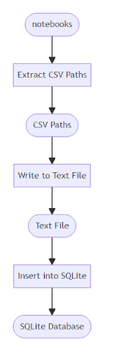
Importing CSV Files into SQLite Database

Function: import_csv_to_sqlite(csv_file_path, conn)

Purpose: Imports a CSV file into an SQLite database.

• It first gets the name of the CSV file without its extension to use as the table name in the database.
• It attempts to read the CSV file into a DataFrame using the read_csv_safely function.
• If the DataFrame is successfully created, it uploads this DataFrame as a new table in the SQLite database, replacing any existing table with the same name.
• It provides feedback on whether the import was successful or skipped due to read errors.

Function: extract_csv_paths_from_notebook(notebook_path, base_path)

Purpose: Extracts paths of CSV files used in a Jupyter notebook.

• Opens the notebook and reads through its content.
• Searches for any line of code that involves reading a CSV file (using pandas).
• Extracts the path of the CSV file mentioned in the code, ensuring it's a full path resolved relative to the notebook’s location.
• Checks if the extracted path exists and adds it to a list if it does; otherwise, it warns about the missing path.

Function: process_files(data_path, db_path)

Purpose: Manages the processing of either a single CSV file, multiple CSV files, or Jupyter notebooks found in a specified directory.

• Connects to the specified SQLite database. If the database does not exist, it will create a new one.
• Checks if the data_path provided is a directory or a specific file:
• If a directory, it processes all CSV files and notebooks found within.
• If a file ends with .csv, it processes just this file.
• If a file ends with .ipynb, it extracts CSV paths from the notebook and processes them.
• If the path isn’t a directory or supported file, it alerts the user.
• Closes the database connection after all files are processed to ensure no resources are left hanging.

https://docs.google.com/document/d/1Y_b1LtPke0WaReWIXPjQ0PE3NtKOwnDEx8oLKD7VM8s/edit

Output : home/gqc/git/gqc/notebooks/db/cctv.db

5/6/2024

nbdev

• nbdev is an open-source system that allows you to fully develop a Python library in Jupyter Notebooks, It's developed by fast.ai
• You can write your code, tests, and documentation all in one place—inside Jupyter Notebooks
• PR is easier with nbdev

https://general.gqc.com/dev/Python/nbdev

https://nbdev.fast.ai/tutorials/tutorial.html

Reflection on my nbdev : add

Mambaforge

On WSL and Ubuntu based systems, GQC uses mambaforge to manage python environments.

Mambaforge allows you to create a new virtualenv with a different python version compared to its initial install. This is a required feature as many AI algorithms have dependencies on certain python versions.

Comments :

Add DRF-video DRF in gqc documentation

Sphinx

more generic documentation generator (it works with all Python code, not just Django applications)

sphinx-doc

Django Rest Framework

• Serialization: DRF provides serializers that allow complex data such as querysets and model instances to be converted to native Python data types that can then be easily rendered into JSON, XML, or other content types. Serializers also provide deserialization, allowing parsed data to be converted back into complex types.

• Browsable API: DRF includes a browsable API that's human-friendly and accessible through a web browser. This allows developers to interact with the API, providing a great tool for debugging and understanding API endpoints.

• Authentication and Permissions: DRF supports various authentication schemes (such as OAuth1a, OAuth2, and others) and has built-in permission classes that can be used to restrict access to APIs based on the requesting user.

1. Models

Django models are Python classes that map to database tables and define the structure of your application's data. Each model class defines fields as class attributes, representing columns in the database. Relationships between models are also defined here.

Example:

_from django.db import models_

_class Book(models.Model):_

_    title = models.CharField(max_length=200)_

_    author = models.CharField(max_length=100)_

_    published_date = models.DateField()_

2. Views

Views process incoming HTTP requests, interact with models, and return appropriate responses. In DRF, views can be function-based or class-based, with APIView or ViewSet as common base classes.

Example (Class-Based View):

from rest_framework.views import APIView

from rest_framework.response import Response

class HelloWorldView(APIView):

    def get(self, request):

        return Response({"message": "Hello, world!"})

3. Serializers

Serializers convert complex data like querysets and model instances to native Python datatypes that can then be rendered to JSON or XML. They also handle data validation and deserialization.

Example:

from rest_framework import serializers

from .models import Book

class BookSerializer(serializers.ModelSerializer):

    class Meta:

        model = Book

        fields = ['id', 'title', 'author', 'published_date']

4. URLs

URLs define the routing system that maps URL patterns to views. This is usually done using the path or re_path functions.

Example:

from django.urls import path

from .views import HelloWorldView

urlpatterns = [

    path('hello/', HelloWorldView.as_view(), name='hello-world'),

]

6. Tests

Tests are essential for validating application functionality. Django provides a test framework that allows you to write unit and integration tests for your API.

Example:

_from rest_framework.test import APITestCase_

_class HelloWorldViewTest(APITestCase):_

_    def test_hello_world(self):_

_        response = self.client.get('/hello/')_

_        self.assertEqual(response.status_code, 200)_

_        self.assertEqual(response.data, {"message": "Hello, world!"})_

7. Apps

An app in Django is a web application that does something, like a blog or a booking system. Each project can contain multiple apps. Each app has its own models, views, serializers, and templates. The app configuration is done in the apps.py file.

Example (AppConfig):

_from django.apps import AppConfig_

_class BooksConfig(AppConfig):_

_    default_auto_field = 'django.db.models.BigAutoField'_

_    name = 'books'_

Created a DRF example : C:\Users\vishwanatha\myproject\myapp

5/7/2024

Parse CSV into SQLite - Redeux

Run the script for 3 different notebook directories:

/home/gqc/git/gqc/gqc-utility-notebooks/nbs/02_CCTV

/home/gqc/git/gqc/gqc-utility-notebooks/nbs/03_Generic\ Utilities

/home/gqc/git/gqc/gqc-utility-notebooks/nbs/04_CCTV\ GIS\ +\ Prediction

Each notebook directory should be its own database, named the following:

**02_CCTV.db3

03_Generic_Utilities.db3

04_CCTV_GIS_Prediction.db3**

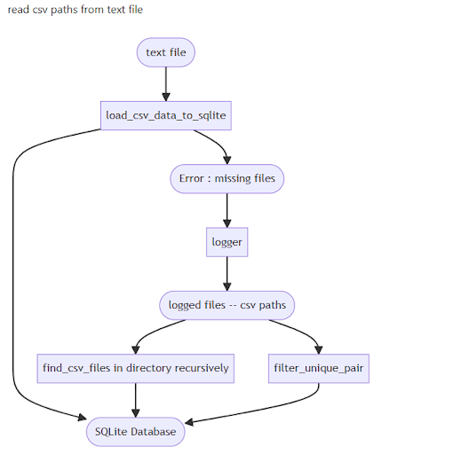
Comments : improve code base add logger to see missing parsed csv files

Mermaid

https://mermaid.js.org/syntax/classDiagram.html \

https://general.gqc.com/dev/diagraming

5/8/2024

Parse CSV into SQLite - Redeux

02_CCTV.db3

Path : /home/gqc/git/gqc/gqc-utility-notebooks/nbs/DB/02_CCTV1.db3

04_CCTV_GIS_Prediction.db3

Path : /home/gqc/git/gqc/gqc-utility-notebooks/nbs/DB/04_CCTV_GIS_Prediction.db3

Notebook-path (key-value)

Path : /home/gqc/git/gqc/gqc-utility-notebooks/nbs/DB/02_CCTV key-pair.db3

Path : /home/gqc/git/gqc/gqc-utility-notebooks/nbs/DB/04_CCTV GIS + Prediction key-pair.db3

This database stores unique pairs of notebook names and CSV paths extracted from notebooks related to CCTV GIS prediction. Each notebook's name is used as the table name, and each table contains pairs of notebook names and associated CSV paths.

Comments :

Two column table notebook name and csv full path

Path : /home/gqc/git/gqc/gqc-utility-notebooks/nbs/DB/02_CCTV key-pair.db3

Path : /home/gqc/git/gqc/gqc-utility-notebooks/nbs/DB/04_CCTV GIS + Prediction key-pair.db3

Intro to dicom (understanding the data)

DICOM files contain both image data and metadata. The image data can be 2D, 3D, or 4D (time series) and includes various modalities such as X-ray, MRI, CT scan, ultrasound, etc.

https://academic.oup.com/jamia/article/4/3/199/832255

https://siim.org/learning/dicom-introduction-data-formats-and-protocol/

How 3d slicer does it?

Unreal>>>>>/unity 3d libraries

https://github.com/tommybazar/TBRaymarcherPlugin

Cuda enabled lGBM (high Priority)

LightGBM training

Polar Coordinates (r,θ):

r: The distance from a central point (the pole or origin) to the target point.

θ: The angle between the positive x-axis and the line segment connecting the pole to the target point, measured counterclockwise.

5/9/2024

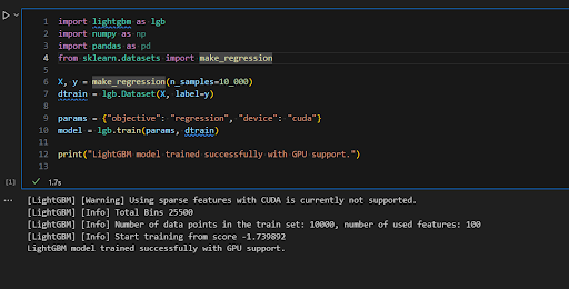
LightGBM using cuda cores

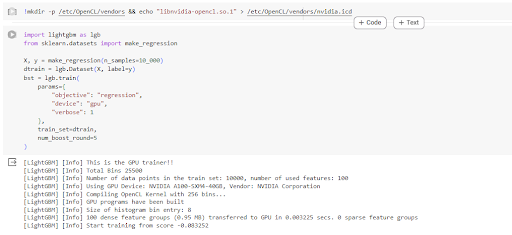
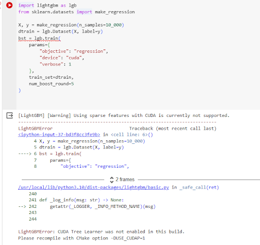
https://lightgbm.readthedocs.io/en/latest/GPU-Windows.html (try in my laptop) after hours

https://stackoverflow.com/questions/57412261/how-can-i-solve-problem-with-installing-lightgbm-gpu-on-windows-10

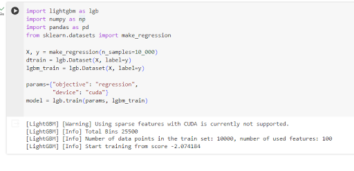
Successful run of LighGBM with cuda cores

https://colab.research.google.com/drive/1_R9mBFAk0C671N6ntIzxov3G0c6V5p2g#scrollTo=nW7Ays1OxUD-

5/10/2024

Convert deepvibe-dsp-c into an Azure Function App

https://github.com/gqc/deepvibe-dsp-c/tree/main

C application that currently runs on a Linux environment, connects to a Timescale database to query saved measurements, and then applies digital signal processing (DSP). want to migrate this functionality to a Function App in Azure?.

Continuing with LGBM with Cuda in notebook 07 on Colab

def create_lgbm_model(model_params_pickle_file):

    with working_directory(CCTV_DIR / BEST_MODEL_PARM_DIR):

        with open(model_params_pickle_file, 'rb') as fp:

            model_params = pickle.load(fp)

    lgbm = lgb.LGBMClassifier(**model_params, random_state=42)

    return lgbm

create_lgbm_model function:

• This function takes a single argument model_params_pickle_file, which is the file path of a pickle file containing the parameters for the LightGBM model.

with open(model_params_pickle_file, 'rb') as fp:

* This opens the pickle file specified by `model_params_pickle_file` in binary read mode (`'rb'`).
* It reads the content of the pickle file into the file pointer `fp`.

model_params = pickle.load(fp)

* This loads the content of the pickle file (presumably containing model parameters) into the variable `model_params`.

lgbm = lgb.LGBMClassifier(model_params, random_state=42)

* This line creates an instance of the LightGBM classifier (`LGBMClassifier`) using the parameters loaded from the pickle file (`model_params`).
* It sets the `random_state` parameter to 42 for reproducibility of results.

model_params["device"] = "cuda"

Suggested update :

def create_lgbm_model(model_params_pickle_file):

    with working_directory(CCTV_DIR / BEST_MODEL_PARM_DIR):

        with open(model_params_pickle_file, 'rb') as fp:

            model_params = pickle.load(fp)

    # Add the device parameter to the model params

    model_params["device"] = "cuda"

    lgbm = lgb.LGBMClassifier(**model_params, random_state=42)

    return lgbm

Update lgbm_param_grid to include the CUDA device parameter

lgbm_param_grid = {"max_depth": [25,50, 75],

                   "learning_rate" : [0.01,0.05,0.1],

                   "num_leaves": [300,900,1200],

                   "n_estimators": [50, 100, 200],

                   "device": ["cuda"]}

5/13/2024 :

CCTV notebook 7

1. Finish mapping material types in notebook 07. Look at Vannary's other code to figure out how they should map.

done

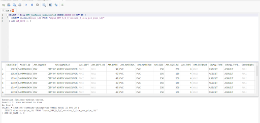
2. Find all pipes missing AM_DATE from the uninspected pipes.

1. Map of uninspected pipes, color coded by material type.

Collimator : update sharepoint

5/14/2024 :

Notebook 12 : make duplicate of notebook 02

Make modifications to handle new data

04_CCTV GIS + Prediction

• 01_GIS+Prediction_DNV_mapping_defects_version_2.ipynb: Combine the correct material, defect, and other metadata from metadata DBs and shape files to prepare: 1. CSVs, 2. shape files ( I need to dive into the details to understand what's going on fully)
• 02_GIS+Prediction_prepare_data_for_defect_prediction_version_2.ipynb: Combines the data from shapefiles and metadata and creates a 'row per pipe' csv with all features to be used in training.
• 03_GIS+Prediction_lightGBM.ipynb: Old notebook for lightGBM, This trains and evaluates lightGBM and writes the predictions to shape files
• 03_RandomForest_xgb_lgbm_catboost.ipynb: Latest nb which identifies the optimal parameters for the prediction model by grid search on random-forest, xgboost, lightGBM. and CatBoost
• 04_GIS+Prediction_compile_results_CCTV_prediction_model.ipynb: Generate ROC AUC curves
• 05_GIS+Predictions_generate_shap_plot.ipynb: Shap plots for identifying important features
• 06_GIS+Predictions_save_the_predictions_to_shape_files.ipynb: Train a model with the selected optimal parameters (one time), save the model, load the model to run on a test set and write the result to shape file.

5/15/2024 :

Notebook 07

Prediction QGIS

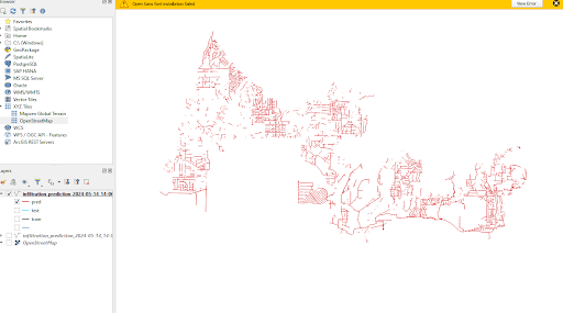
Test & Train QGIS

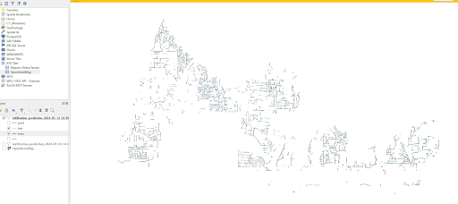
Comments : view train,test and pred shape files separately

Table for paths for every csv?

Update documentation on openvpn

5/16/2024 :

Train :

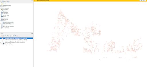
Test :

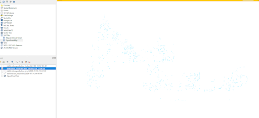
Pred :

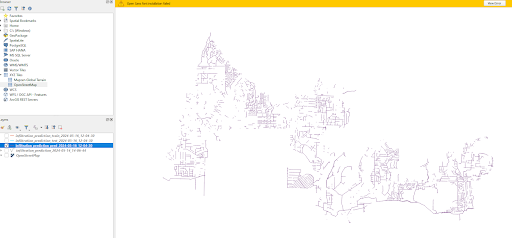
Uninspected_pred:

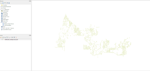
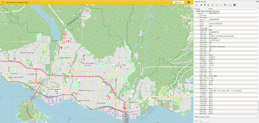
5/17/2024

RKSP :

what is the difference between a .dcm file and a dicom folder without .dcm files

Storage Method: A .dcm file is a single file, while a DICOM folder without .dcm files uses a directory structure to organize multiple related files.

File Content: .dcm files contain both image and metadata in one file, whereas a DICOM folder can split this information across multiple files with different formats.

Usage Context: .dcm files are suited for simpler scenarios or individual image transfers, while DICOM folders are used for more complex datasets that require a structured approach to manage multiple images and associated data.

Can you convert the folder into a single .dcm file?

DICOM Toolkit (DCMTK):

DCMTK is a collection of libraries and applications for working with DICOM files. You can use the dcmmkdir tool to create DICOMDIR files from a set of DICOM files, and other tools in the suite to manage and convert files

GDCM (Grassroots DICOM)

How to convert brain DICOM image slices into 3D representations?

InVesalius: This open-source software generates 3D medical imaging reconstructions from a sequence of 2D DICOM images (CT or MRI). It works on Windows, Linux, and macOS. InVesalius supports various medical imaging modalities and provides features like segmentation, 3D surface creation, and volume rendering.

workflow for prototyping

InVesalius for 3D Reconstruction:

1. InVesalius is primarily designed for medical imaging reconstruction. It takes DICOM files (such as CT or MRI scans) and generates 3D models (usually in STL format).
2. Once you have the 3D model from InVesalius, you can export it as an STL file.
3. However, Unreal Engine typically uses other formats (such as FBX or OBJ) for assets. So, you’ll need to convert the STL file to a compatible format using additional software (e.g., Blender).
4. Blender for Format Conversion:
5. Import the STL file generated by InVesalius into Blender (a free and powerful 3D modeling software).
6. In Blender, you can further refine the model, adjust materials, and optimize it for real-time rendering.
7. Export the model from Blender in a format that Unreal Engine supports (e.g., FBX).
8. Unreal Engine Integration:
9. Import the FBX (or other compatible format) into Unreal Engine.
10. Set up materials, lighting, and physics properties within Unreal Engine.
11. Use the 3D model as part of your game or visualization project.
12. Remember that this workflow involves multiple steps, but it allows you to create detailed and accurate 3D models from medical imaging data and use them in Unreal Engine projects.
13. Unity supports FBX (Filmbox) files. The FBX format is widely used in 3D graphics applications for storing complex models, animations, and textures. Unity's support for FBX files allows developers to import 3D models and animations created in various 3D modeling software like Autodesk Maya, Blender, and 3ds Max directly into Unity.

Comments : Pickle and Joblib

Pickle is a versatile choice for serializing Python objects, while Joblib is optimized for handling NumPy arrays efficiently and provides additional features for parallel processing

Uc-report : Getting Started with Embedded Linux Security

webinar link : attachment

Full Doulos portfolio doulos-training

Authorised Training for AMD doulos-amd

Using AMD High Level Synthesis to supercharge your design performance hlsworkshop

How to Accelerate both your FPGA Application & Productivity FPGA

Designing with AMD Versal AI Engines: Quick Start

Includes courses covering: Versal / Vitis / Kria / Alveo FPGA Design / Embedded Systems / DSP / Connectivity

FREE Live Online Versal Adaptive SoCs: Quick Start workshop versalqsworkshop

Doulos Live Online Training doulos-iot

Viewtify unreal engine 4 / 5

medical image (DICOM image) viewer that can instantly synthesize high-quality 3DCG in real time from CT / MRI images.

viewtify

jtcvstechniques.org

TASKS :

Jira task: note all the findings from WEBINAR

Comments : how do we make our embedded ubuntu version 22 more secure?

Jira task : store and document “AI_model_save_load_from_pkl.ipynb” use nbdev

Pickle vs joblib :

The choice between pickle and joblib depends on the specific use case and the type of data you are dealing with. Here's a more detailed comparison to help determine which is better for your needs:

When to Use Pickle

Advantages:

• Standard Library: No need for additional installations; pickle is included with Python.

• Versatility: Can serialize a wide variety of Python objects, including custom classes and complex data structures.

• Simple API: Easy to use with straightforward dump and load methods.

Disadvantages:

• Performance: Can be slower with large datasets, particularly those containing numpy arrays.
• Security: Loading pickled data from untrusted sources can be a security risk because it can execute arbitrary code during unpickling.

Best For:

• General-purpose serialization when performance is not a critical concern.

• Serializing and deserializing Python objects that are not primarily large numpy arrays or numerical data.

When to Use Joblib

Advantages:

• Performance: Optimized for large numpy arrays and numerical data, leading to faster read and write times compared to pickle.

• Compression: Supports compression, which can significantly reduce file size.

• Memory Mapping: Allows for efficient storage and access to large data through memory mapping.

Disadvantages:

• Dependencies: Requires installation of the joblib library.

• Specialized: Primarily optimized for numpy arrays and numerical data; might not offer significant advantages for other types of objects.

Best For:

• Working with large numerical datasets, especially those containing numpy arrays.

• When performance (speed of serialization/deserialization) is a critical factor.

• Situations where reducing file size through compression is beneficial.

Summary

• Use pickle if: You need a standard, versatile serialization method that can handle a wide range of Python objects and do not have significant performance requirements.

• Use joblib if: You are working with large numerical datasets, require faster serialization/deserialization, or need efficient storage and access to large data through memory mapping and compression.

In summary, pickle is better for general-purpose use, while joblib is better for performance-sensitive applications involving large numerical data.

5/20/2024 :

included additional data in df_pred DataFrame

df_pred_final = pd.DataFrame({'pipe_id': to_be_pred_df['ASSET_ID'],

                              'true_I': final_pred_bool,

                              'pred_I': final_pred,

                              'segment_material': to_be_pred_df['AM_MATER00'],

                              'age': formatted_to_be_pred_df['age'],

                              'pipe_length': to_be_pred_df['ASB_LENGTH'],

                              'data': 'pred'})

uninspected pipes :

SELECT DISTINCT p1.'ASSET_ID,C,12'

FROM SanMain p1

LEFT JOIN row_per_pipe_id p2 ON p1.'ASSET_ID,C,12' = p2.'pipe_id'

WHERE p2.pipe_id IS NULL;

SELECT * FROM `SanMain` p1 where p1.'ASSET_ID,C,12' NOT IN (SELECT p2.'pipe_id' FROM 'row_per_pipe_id' p2)

Total rows loaded : 4990

5/21/2024 :

uninspected pipes :

SELECT * FROM `SanMain` p1 where p1.'ASSET_ID,C,12' NOT IN (SELECT p2.'pipe_id' FROM 'row_per_pipe_id' p2)

Total rows loaded : 4990

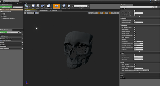
Importing FBX to unreal engine

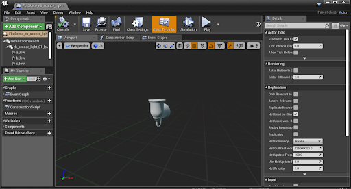
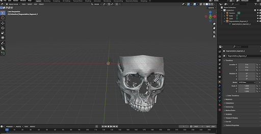
Importing STL file to blendor :

Importing FBX file to unreal_engine

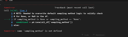
Notebook 07 :

Infiltration_prediction_2024-05-21_15-50-46.shp rectangular co_ordinates (3:52)

5/22/2024

data for power BI

SELECT *

FROM `row_per_pipe_id` p1

WHERE p1.pipe_id NOT IN (

SELECT p2.`pipe_id,C,80`

FROM `train` p2

UNION

SELECT p3.`pipe_id,C,80`

FROM `test` p3

);

Output : 35 rows were outputed

1. Provided the files for uninspected_infiltration_rectangle/polar and uninspected_structural_rectangle/polar.
2. Helped Iniyaa with her JSON to XLSX conversion.
3. Switched to nbdev but encountered the same issues listed by Melissa from yesterday (on hold).
4. Switched back to Melissa's task and provided her with the following numbers:

*** Total pipes : 7832

• Total inspected pipes : 3673
• Total uninspected pipes : 4990
• Pipes used in training: 2910
• Pipes used in testing: 728**

**total inspected pipes : 3673

(updated count ): train pipes : 2910

test pipes : 728

distinct inspected pipes : 2853

distinct test pipes : 693

distinct train pipes : 2380 **

. Working with help of Melissa to perform QA and ensure the numbers are correct.

5/23/2024

Moving Notebook-07 to Python Script

CCTV-56

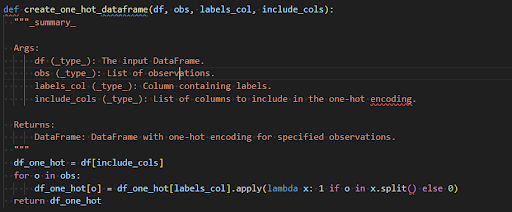
SPHINX :

Sphinx-GQC

I also looked on Dropbox and this was also the answer there as well. We use the pydocstyle for commenting so that must be where I am getting pydocs.

Documentation​

• Documentation for Python code is generated from "docstrings". Refer to Customize VS Code for more information on plugins to facilitate the writing of docstrings.
• The linter "pydocstyle" can be used to check for errors in docstrings.
• After documenting a codebase with docstrings, one of two paths can be taken to generate documentation:
• Django built-in admindocs (Specifically for Django)
• Sphinx
• You will want to use Sphinx.
• Please follow the instructions on the website for generating Sphinx documentation.
• I would follow the Generate md files with Sphinx instructions rather than the html ones.

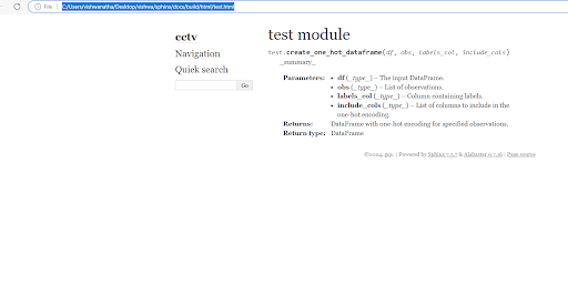
tried documenting a test code using Sphinx and viewed it in HTML

5/24/2024

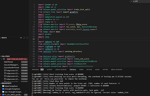
Moving notebook to python script :

5/28/2024

Moving notebook to python script

5/29/2024

Moving notebook to python script

infiltration_rectangular model training

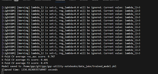
Load Saved Model :

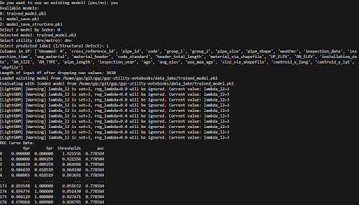
5/30/2024

Moving notebook to python script

adding additional functionalities

5/31/2024 :

Moving notebook to python script :

Halted (MSI server Maintenance)

Switching to RKSP

RKSP

medivis

medivis-stl-importer

On-premise IT deployment. No cloud. No PHI stored.

Patient data never leaves the hospital firewall. A seamless, secure HIPAA compliant PACS integration.

connecting AI to IOT Applications

• AI-IOT

ITK smoothing filter with vtk view

The code reads a DICOM series from a specified directory using ITK, processes the image with a smoothing filter, converts the ITK image to a VTK image, and visualizes it using VTK. The main function orchestrates these steps to display the smoothed DICOM image in a VTK rendering window.

ITK-Docs

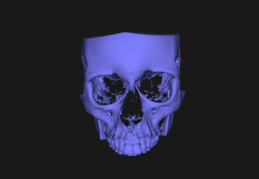
STL view with VTL

Rendering STL file exported from 3D-slicer and used vtk library ro render the skull

6/3/2024 :

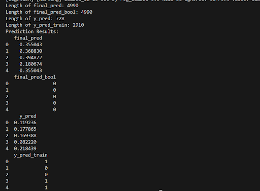
Moving notebook to python script :

• Generate Predictions for Test Set
• Generate Predictions for Training Set
• Generate Final Predictions

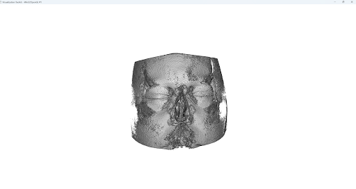
Dicom to 3D using itk and vtk replicating 3d slicer :

Sure, here's a brief explanation of each function in the code:

1. load_dicom_series(directory):

   • Loads a series of DICOM images from the specified directory using SimpleITK.

   • Returns the images as a 3D volume.

2. resample_image(image, new_size, new_spacing):

   • Resamples the given image to the specified new size and spacing.

   • Uses linear interpolation to adjust the image dimensions, ensuring consistency across different views.

3. apply_threshold(image, lower_threshold, upper_threshold):

   • Applies a binary threshold to the image, setting voxel values within the specified range to 1 and others to 0.

   • Helps to highlight relevant structures by filtering out irrelevant parts of the image.

4. crop_image(image, start, size):

   • Crops the given image to a specified region defined by the start coordinates and size.

   • Focuses on a particular area, such as the face region, to reduce unnecessary data.

5. render_volume(image):

   • Converts the SimpleITK image to a VTK image and sets up volume rendering properties.

   • Renders the 3D volume using VTK, allowing visualization of the combined images.

LGBM with cuda core local :

6/4/2024 :

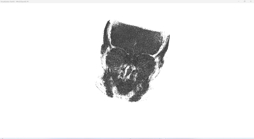
Increased voxel intensity to view the skull

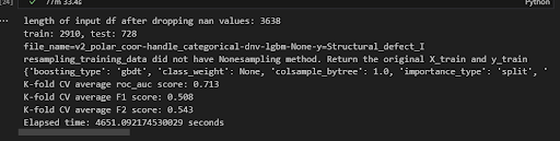
Trained structural_polar :

6/5/2024 :

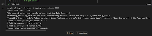
infiltration_polar

6/6/2024 :

Wandb

CCTV DNV presentation

6/7/2024 :

Model training without negative length - Rectangular Co-ord :

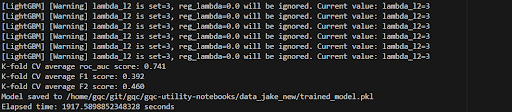
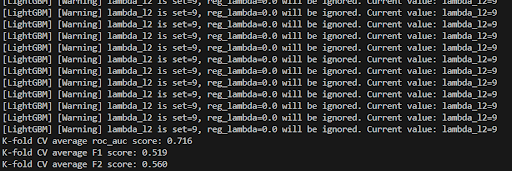
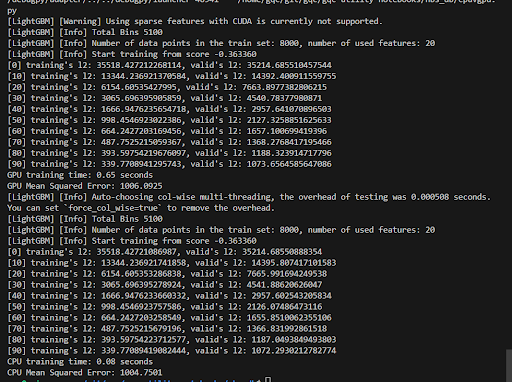
CPU vs CUDA training metrics

RKSP : Skull Stripping

yale-medicine

skull-sripping-preprocessing

extract-skull-from-dicom

6/10/2024 :

• I will be checking LGBM-GPU model training and its predictions, will ask jake for help
• After this, I will continue to work on the notebook and aim to complete the remaining tasks
• .Save as Shapefile:
  • Save the GeoDataFrame as a Shapefile for further analysis and use.

• Finally, I will switch to the RKSP project and start exploring the following :
  • interacting with the skull/soft tissue model, including rotating and zooming, adjusting transparency, slicing through specific planes, and using the cursor to cut or remove tissue.

LGBM cuda error

CPU

{'boosting_type': 'gbdt', 'class_weight': None, 'colsample_bytree': 1.0, 'importance_type': 'split', 'learning_rate': 0.1, 'max_depth': 30, 'min_child_samples': 20, 'min_child_weight': 0.001, 'min_split_gain': 0.0, 'n_estimators': 50, 'n_jobs': None, 'num_leaves': 30, 'objective': 'binary', 'random_state': 42, 'reg_alpha': 0.0, 'reg_lambda': 0.0, 'subsample': 1.0, 'subsample_for_bin': 200000, 'subsample_freq': 0, 'lambda_l2': 3, 'scale_pos_weight': 5.751724137931035}

CUDA

{'boosting_type': 'gbdt', 'class_weight': None, 'colsample_bytree': 1.0, 'importance_type': 'split', 'learning_rate': 0.1, 'max_depth': 30, 'min_child_samples': 20, 'min_child_weight': 0.001, 'min_split_gain': 0.0, 'n_estimators': 50, 'n_jobs': None, 'num_leaves': 30, 'objective': 'binary', 'random_state': 42, 'reg_alpha': 0.0, 'reg_lambda': 0.0, 'subsample': 1.0, 'subsample_for_bin': 200000, 'subsample_freq': 0, 'lambda_l2': 3, 'scale_pos_weight': 5.751724137931035, 'device': 'cuda'}

• I used the same parameters as those in the .pkl file to train two models using LGBMClassifier. These models were trained on a demo LightGBM dataset to compare CPU vs GPU performance. Both models were accurate, and the predictions were the same.

Parameters used:

python

{

'boosting_type': 'gbdt',

'class_weight': None,

'colsample_bytree': 1.0,

'importance_type': 'split',

'learning_rate': 0.1,

'max_depth': 30,

'min_child_samples': 20,

'min_child_weight': 0.001,

'min_split_gain': 0.0,

'n_estimators': 50,

'n_jobs': None,

'num_leaves': 30,

'objective': 'binary',

'random_state': 42,

'reg_alpha': 0.0,

'reg_lambda': 0.0,

'subsample': 1.0,

'subsample_for_bin': 200000,

'subsample_freq': 0,

'lambda_l2': 3,

'scale_pos_weight': 5.751724137931035,

'device': 'cuda'  # For GPU training

}

• Both the CPU and GPU models provided identical predictions and demonstrated high accuracy on the test set.

• However, when using the same parameters with the CCTV dataset, I encountered errors. Further investigation is needed to understand why the same parameter set is causing issues in this specific context.

• This summary now reflects the successful training and evaluation on a demo dataset and mentions the issues encountered with the CCTV dataset.

LGBM-cuda

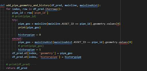
Added Geo Data Frame :

RKSP :

Horus-intro

creating-3d-reconstruction-your-patients-ct-scan

horosproject

anatomical-models-finite-element-analysis

6/12/2024 :

Trained new models on updated inputs

Infiltration rectangular

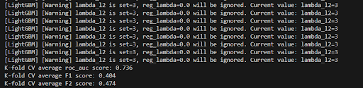
K-fold CV average roc_auc score: 0.736

K-fold CV average F1 score: 0.404

K-fold CV average F2 score: 0.474

Structural rectangular

K-fold CV average roc_auc score: 0.715

K-fold CV average F1 score: 0.520

K-fold CV average F2 score: 0.560

6/13/2024 :

Documenting notebook_07 using sphinx

6/14/2024 :

CCTV py documenting

CCTV-ML mermaid

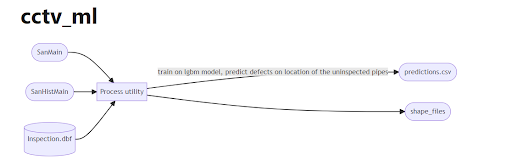
6/17/2024 :

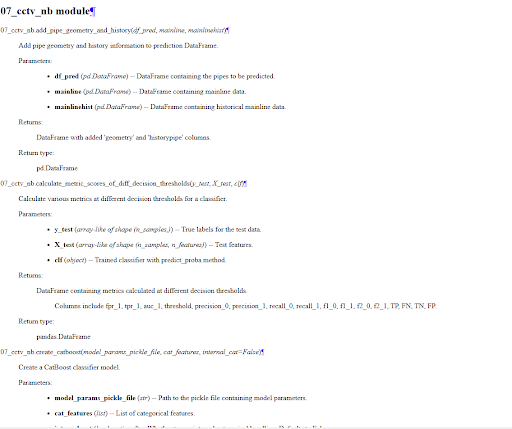
Implemented os.join() for notebook 07

Sphinx Output Notebook 07

UC Report : Cybersecurity for the Water and Wastewater Sector

article link

Comments on Documentation

1. The document doesn't provide enough guidance on how to deal with legacy systems that can't be patched or updated. It should include detailed strategies for mitigating risks associated with these older systems.

2. While the document talks about the need for encryption, it doesn't specify which standards or protocols should be used, like AES-256 or TLS 1.3.

3. The document references several standards (e.g., NIST, AWWA) but doesn't connect them to specific sections or show detailed examples of how to apply them in practice.

4. The document is mostly theoretical and lacks practical examples or case studies that show how to successfully implement the recommended practices. \

Recommendation: Add sections on implementing continuous training programs, including phishing simulations, regular security updates, and best practices for all employees.

6/18/2024 :

Horus Repo Deepdive

Horus-Repo

Webassembly

6/19/2024 :

Epanet

Epanet-Engine

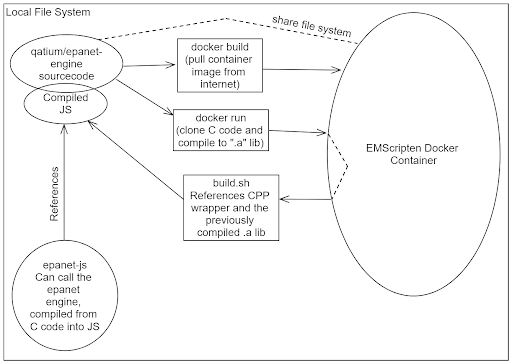
Official docker docs

Official docker docs: link

docker-walkthrough

This one looks really good: Docker-article

GPU for LGBM

Jira-ticket

lightgbm-docs

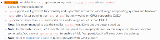
Trained model with GPU support

K-fold CV average roc_auc score: 0.736

K-fold CV average F1 score: 0.402

K-fold CV average F2 score: 0.470

GPU VS CPU Predictions

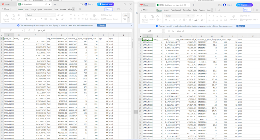
model_params['gpu_use_dp'] = True is added to enable 64-bit floating-point precision on the GPU

6/20/2024 :

RKSP : 2D DICOM to 3D Model Web Application

1. Frontend (React.js)

• Components:
  • FileUpload Component:
    • Allows users to upload DICOM files.
  • ThreeDViewer Component:
    • Visualizes the generated 3D models using three.js.

2. Backend (Django with DRF)

• Models:
  • DicomFile: Stores information about uploaded DICOM files.
• Serializers:
  • DicomFileSerializer: Converts model instances to JSON.
• Views:
  • DicomFileViewSet: Handles file uploads.
• URL Routing:
  • API endpoints for file upload and model retrieval.

3. Processing and Visualization (C++ with ITK and VTK)

• DICOM File Handling and 3D Model Generation:

  * Use ITK for image handling and VTK for 3D model generation.
  * Implement a local C++ application to handle the processing.

  UPDATE: Utilize existing C++ Libraries. Potentially build the C++ codebases into JS libraries using "emcscripten" (or whatever it was called).

• Local Processing:

  * Ensure all processing is done locally on the user's machine.

  UPDATE: Ensure all processing is done locally in the user's browser.

• Data Transfer:

  * Transfer the generated 3D model to the web application for visualization

  UPDATE: There shouldn't be any data transfer. All data should stay in the user's browser environment.

  UPDATE: Ensure all processing is done locally in the user's browser.

Trying VTK.js

6/21/2024 :

RKSP : VTK.js

npx cross-env EXAMPLE=image-slicing.js webpack-dev-server --mode=development

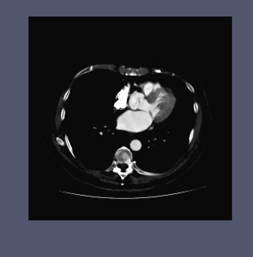
Image Slicing.js

Volume-Transfer.js

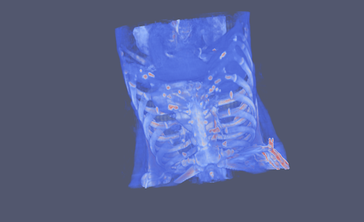
6/24/2024 :

widgets.js

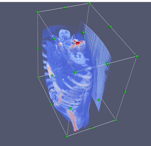
6/25/2024 :

Image Server

cyber-security summit

cybersecuritysummit

6/26/2024 :

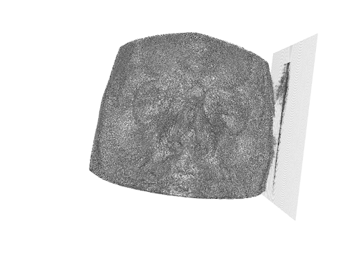
Dicom to 3D

One plane

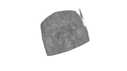
3 planes

6/27/2024 :

RKSP Project Overview and Tools used

6/28/2024 :

Improved Volume transfer using python

RKSP

Volume transfer

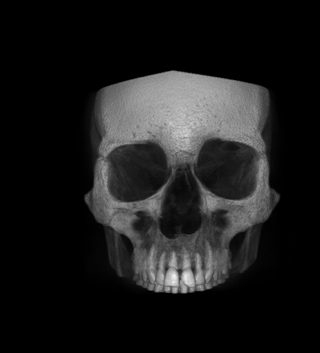
Drilled

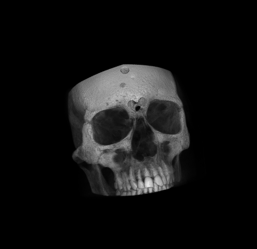
7/1/2024 :

VTK rendering

• Compared single-plane and three-plane VTK rendering.
• Tried running Kitware vtk.js locally with Elizabeth DICOM files couldnt load.
• Successfully ran VolView locally.
• Enhanced the existing Python 3D structure rendering.
• Performed drill simulations in the 3D structures.

7/2/2024 :

TASKS

• hack wall view, to implement drilling functionality how do we reprsent,can it be other than cylinder, not chopping it, scapel?

• move the tool around, pre simulated cut?, implementation?, temporary object

• how can i make api calls to monai?, what data format does the api need?

• unreal? format works, assets?, nvdia monai volume representation

7/3/2024 :

RKSP Exploration

unreal-drilling-hole-realtime

Delivering Surgical Training 5x Faster with VR

precisionostech-vr-training

Game : surgery simulator

ITK-Third_Party_Applications

mevislabdownloads

NOTES :

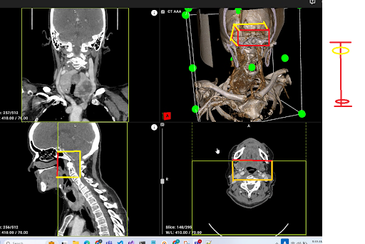
7/5/2024 :

RKSP Exploring Volview

Retrieve the existing cropping planes from the state.

Check if the actor is inside the planes.

Set the visibility based on the check.

Request render to update the view.

Inputs:

lpsPlanes: The planes defining the cropping box.

view: The view object containing the renderer and actors.

state: The state object containing the current cropping planes.

imageMetadata: Metadata containing orientation information.

Processes:

Retrieve cropping planes: Get the current cropping planes from the state.

Check actor bounds: Determine if each actor is within the cropping planes.

Set visibility: Set the visibility of each actor based on whether it is inside the cropping planes.

Request render: Request the view to render the scene with updated visibility settings.

Outputs:

Existing cropping planes: The current cropping planes retrieved from the state.

Actor inside check: The result of checking if each actor is within the cropping planes.

Visibility set: The visibility of each actor updated based on the cropping planes.

Updated rendering: The view is rendered with actors inside the cropping box made invisible and those outside visible.

7/8/2024 :

Volview

Exploring Volview

7/9/2024 :

vue.js debugging

• vue.js debugging using vstudio : link

7/10/2024 :

VOLVIEW presentation

• I have included the video of VolView that we previewed during our meeting.

7/11/2024 :

Notes from VTK

• Intresting vtk thread reconstruction-of-cortical-brain-surface-in-3d using vtk

• vtk.js with vue.js link

• Creating a new class in vtk.js link

Widget Architecture Overview link

Developing Widgets link

Widget box with UI link

Widget box with cropping link

Tutorials : link

tutorial link

Apache Licence

7/12/2024 :

VTK Widget handles

paint-widget

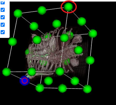
Tasks

1. Look into VTK book
   • Look into VTK (Visualization Toolkit) Book.
   • Document findings and potential solutions.

2. Send a Message for Presets to Rijul
   • Draft a message to Rijul regarding the presets.

3. VTK/Volview GitHub Issues
   • add GitHub issues for the scooping tool link.
   • FPS TPS issue link
   • inverse-cropping-widget-thread
   • Debugging Specific Example in VTK.js using vscode thread

7/15/2024 :

Try Changing the behaviour of the existing cropping widget

task

• change the behaviour of the existing cropping widget

Locate and Modify the Shader:

• Locate the VolumeMapper shader in the vtk.js source code.

• Modify the fragment shader to handle inverse cropping.

• Integrate the Shader Changes:

• Ensure the modified shader is used in your vtk.js example.

• Pass the cropping planes to the shader.

• post the question in forum

• vtk macro? explore track my progress

7/16/2024 :

01_GIS+Prediction_DNV_mapping_defects_version_2.ipynb

SHAPE_FILE_DIR

sanmain = '/home/gqc/git/gqc/gqc-utility-notebooks/data/shapefiles/SanMain_shp/SanMain.shp'
sanfitting = '/home/gqc/git/gqc/gqc-utility-notebooks/data/shapefiles/SanFitting_shp/SanFitting.shp'
sanmainhist = '/home/gqc/git/gqc/gqc-utility-notebooks/data/shapefiles/SanHistMain_shp/SanHistMain.shp'

PACP & WRC

PACP_videos = '/home/gqc/git/gqc/gqc-utility-notebooks/data/condition_data/list_730_PACP_videos_in_CCTV_Details.csv'
all_conditions_wrc_1066 = '/media/gqc/T7/cctv/dnv/data/wrc_1066/temp/all_conditions.csv'

CONDITION_DATA csv

cctv_header = '/home/gqc/git/gqc/gqc-utility-notebooks/data/condition_data/CCTV_Headers.csv'
cctv_detail = '/home/gqc/git/gqc/gqc-utility-notebooks/data/condition_data/dnv_B_C_condition_data_with_remarks_col.csv'
cctv_detail_full = '/home/gqc/git/gqc/gqc-utility-notebooks/data/condition_data/CCTV_Details_sorted_by_jobnumber_distance_code_edit.csv'
cctv_header_81 = '/home/gqc/git/gqc/gqc-utility-notebooks/data/condition_data/combined_pipe_properties_84videos.csv'
cctv_detail_81 = '/home/gqc/git/gqc/gqc-utility-notebooks/data/condition_data/dnv_pacp_A_81_condition_data.csv'

list of videos

list_81_videos = pd.read_csv('DNV_PACP_81videos_edit.csv')
list_videos = pd.read_csv('DNV_PACP_711_out_5238videos.csv')

OUTPUT_SHAPE_FILE_DIR

DNV_81_code_points = '/home/gqc/git/gqc/gqc-utility-notebooks/data/output_shape_files/defect_location_version_2/DNV_81_pacp_code_points.shp'
DNV_B_C_code_points = '/home/gqc/git/gqc/gqc-utility-notebooks/data/output_shape_files/defect_location_version_2/DNV_B_C_pacp_wrc_code_points.shp'

inspection info csv

inspection_info_DNV_A_ '/home/gqc/git/gqc/gqc-utility-notebooks/data/feature_engineering_data/inspection_info_DNV_A_version_2.csv'
inspection_info_DNV_B_C_version_2  '/home/gqc/git/gqc/gqc-utility-notebooks/data/feature_engineering_data/inspection_info_DNV_B_C_version_2.csv
condition_data_DNV_B_C_version_2   '/home/gqc/git/gqc/gqc-utility-notebooks/data/feature_engineering_data/condition_data_DNV_B_C_version_2.csv'

assign_pacp_group_labels(code):

• Assigns PACP group labels to defect codes.

assign_wrc_group_labels(code):

• Assigns WRc group labels to defect codes.

assign_stmh_fnmh_from_upmh_dnmh(header_df, upstream_col, downstream_col, direction_col):

• Determines start and finish manholes based on inspection direction.

assign_upmh_dnmh_from_stmh_fnmh(header_df, startmh_col, finishmh_col, direction_col):

• Determines upstream and downstream manholes based on start and finish manholes.

assign_upmh_dnmh_from_stmh_fnmh_with_nan_direction(header_df, manhole_shapefile, startmh_col, finishmh_col, direction_col, manhole_col):

• Assigns upstream and downstream manholes when direction is missing, using manhole invert elevations.

rename_columns(header_df, list_column_name, list_new_column_name):

• Renames columns in the DataFrame.

get_upstream_and_downstream_pipes_via_mh(header_df, manhole_shapefile, sanitary_shapefile, manhole_col, sanitary_col, pipe_id_col, upstream_col, downstream_col):

• Determines upstream and downstream pipes using manhole positions.

get_upstream_and_downstream_pipes_via_video_name(header_df, sub_header_df, sanitary_shapefile, sanitary_col, pipe_id_col, direction_col, addition_shape):

• Determines upstream and downstream pipes using video names.

assign_case_for_defect_dist(direction, upstream_pipe, downstream_pipe, startmh, finishmh, sanmain, sanmain_col):

• Determines the case for defect distance calculation based on inspection direction and pipe positions.

list_pipe_segments_corresponding_to_condition_data(report_name, end_survey_dist, CASE, start_pipe, start_manhole, sanmain, sanfitting, sanmain_col, sanfitting_col, multi_pipes, debug):

• Lists pipe segments corresponding to condition data for defect mapping.

dist_from_current_pipe_first_point(CASE, defect_dist_from_first_manhole, pipes_length):

• Calculates the distance from the current pipe's first point to the defect.

pipe_segment_material_dist(mmc, end_survey_dist, distance_col, prev_material_col, new_material_col):

• Determines pipe segment material distribution along the surveyed distance.

create_defect_point(header_df, subheader, detail_df, sanmain, reference_id_col_header, reference_id_col_detail, direction_col_header, code_col_detail, distance_col_detail, sanmain_col, multi_pipes):

• Creates defect points based on the header and detail data.

7/17/2024 :

02_GIS+Prediction_prepare_data_for_defect_prediction_version_2.ipynb

Mainline

SanMain.shp = '/home/gqc/git/gqc/gqc-utility-notebooks/data/shapefiles/SanMain_shp/SanMain.shp'
SanHistMain.shp = '/home/gqc/git/gqc/gqc-utility-notebooks/data/shapefiles/SanHistMain_shp/SanHistMain.shp'

DATA A

 DNV_81_pacp_defect_points_material_edit.shp = '/home/gqc/git/gqc/gqc-utility-notebooks/data/output_shape_files/defect_location_version_2/DNV_81_pacp_defect_points_material_edit.shp'
 DNV_81_pacp_code_points_material_edit.shp = '/home/gqc/git/gqc/gqc-utility-notebooks/data/output_shape_files/defect_location_version_2/DNV_81_pacp_code_points_material_edit.shp'
 inspection_info_DNV_A_version_2.csv = '/home/gqc/git/gqc/gqc-utility-notebooks/data/feature_engineering_data/inspection_info_DNV_A_version_2.csv'

DATA B

 dnv_pacp_A_81_condition_data.csv = '/media/gqc/unionsine1/VS_Research/CCTV/DNV/Data/condition_data_csv/dnv_pacp_A_81_condition_data.csv'
 condition_data_DNV_B_C_version_2.csv = '/home/gqc/git/gqc/gqc-utility-notebooks/data/feature_engineering_data/condition_data_DNV_B_C_version_2.csv'
 DNV_B_C_pacp_wrc_defect_points_material_edit.shp = '/home/gqc/git/gqc/gqc-utility-notebooks/data/output_shape_files/defect_location_version_2/DNV_B_C_pacp_wrc_defect_points_material_edit.shp'
 inspection_info_DNV_B_C_version_2.csv = '/home/gqc/git/gqc/gqc-utility-notebooks/data/feature_engineering_data/inspection_info_DNV_B_C_version_2.csv'
 DNV_B_C_pacp_wrc_code_points_material_edit.shp = '/home/gqc/git/gqc/gqc-utility-notebooks/data/output_shape_files/defect_location_version_2/DNV_B_C_pacp_wrc_code_points_material_edit.shp'

stats

 dnv_B_C_condition_data = '/home/gqc/git/gqc/gqc-utility-notebooks/data/condition_data/dnv_B_C_condition_data.csv'

 data/Video_Lists/{group}.csv Loop 1 = '/home/gqc/git/gqc/gqc-utility-notebooks/data/Video_Lists/{group}.csv'
 PACP_270/Data/Video_Lists/{group}.csv Loop 2 = '/home/gqc/git/gqc/gqc-utility-notebooks/data/PACP_270/Data/Video_Lists/{group}.csv'

 video_list = '/home/gqc/git/gqc/gqc-utility-notebooks/data/Video_Lists/dnv_pacp_A_81_01_81.csv'

 dnv_pacp_A_81_condition_data = '/home/gqc/git/gqc/gqc-utility-notebooks/data/condition_data/dnv_pacp_A_81_condition_data.csv'

output

 input_DNV_A_B_C_version_3_(row_per_pipe_id).csv = '/home/gqc/git/gqc/gqc-utility-notebooks/data/feature_engineering_data/input_DNV_A_B_C_version_3_(row_per_pipe_id).csv'

7/18/2024 :

03_RandomForest_xgb_lgbm_catboost.ipynb

04_GIS+Prediction_compile_results_CCTV_prediction_model.ipynb

05_GIS+Predictions_generate_shap_plot.ipynb

06_GIS+Predictions_save_the_predictions_to_shape_files.ipynb

7/19/2024 :

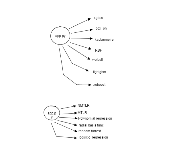
Key Points

• pipe-breaks: Handles initial data processing and model training.
• loe-coe-app: Simplifies user interaction with models for prediction tasks.
• pipe-breaks-transfer-learning: Enhances models through transfer learning and additional testing.

7/22/2024 :

volview-documentation, github repo

https://general.gqc.com/people/Vishwanatha/RKSP/Volview

7/23/2024 :

https://general.gqc.com/people/Vishwanatha/RKSP/vtk.js

https://general.gqc.com/people/Vishwanatha/RKSP/gqc-vtk

7/24/2024 :

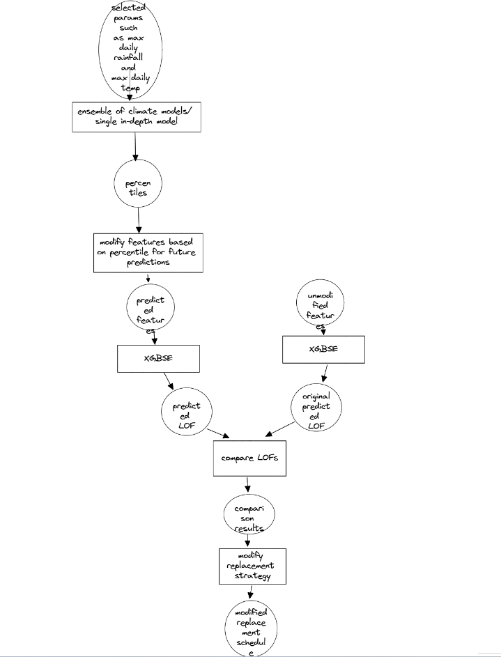
Data Selection

• Select parameters such as maximum daily rainfall and maximum daily temperature.

Modeling

• Use an ensemble of climate models or a single in-depth model to generate percentiles.

Feature Modification

• Modify features based on percentiles for future predictions.

Prediction with Modified Features

• Use XGBoost (XGBASE) to predict the modified features' expected life of the feature (LOF).

Prediction with Original Features

• Use XGBoost (XGBASE) to predict the original feature's LOF.

Comparison

• Compare the predicted LOFs from both modified and original features.

Modification Strategy

• Based on comparison results, modify the replacement strategy.

Output

• Generate a modified replacement schedule based on the updated strategy.

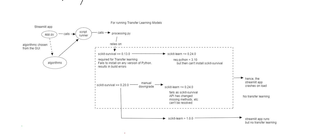
Streamlit App

• app.py calls a script runner.
• The script runner calls processing.py.
• The algorithms chosen from the GUI are used by the script runner.

Dependency Issues

• scikit-survival == 0.13.0 is required for transfer learning but fails to install on any Python version, causing build errors. This version relies on scikit-learn <= 0.24.0.
• scikit-learn <= 0.24.0 requires Python < 3.10, which conflicts with other requirements.
• Manual downgrade to scikit-survival == 0.20.0 and scikit-learn <= 0.24.0 results in missing methods and API changes, leading to failures.
• Using scikit-learn > 1.0.0 allows the Streamlit app to run but disables transfer learning functionality.

Current Situation

• With scikit-survival == 0.13.0 and scikit-learn <= 0.24.0, the Streamlit app crashes on load.
• With scikit-survival == 0.20.0 and scikit-learn <= 0.24.0, transfer learning doesn't work due to API changes and missing methods.
• With scikit-learn > 1.0.0, the Streamlit app runs, but transfer learning is not supported.

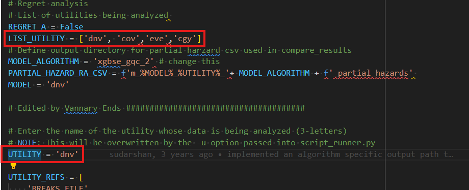
loe-coe

DNV Utility

Sqlite

• As of 07/25/2024
• the app supports only the DNV utility, uses an SQLite database to store results, and has all functionality combined in a single script.

7/25/2024 :

TODO

• Run different utilities - add cov and check (utility)
• Srujana had a TODO to document the loe-coe app: https://general.gqc.com/people/Srujana/2023/august/week_1

Pavan documented the code changes to the app: https://general.gqc.com/people/Pavan/Daily%20Updates/2023/November%202023/Week%204

But otherwise there is basically no documentation for this app. I (Jake) do not know what LOE or COE mean, nor do I know what this app is supposed to do

XGBSE

• It imports and preprocesses the data.
• Selects relevant columns and splits the data into training and validation sets.
• Converts the data into the required format for XGBoost.
• Trains the model using the training data.
• Predicts survival probabilities using the validation data.
• Evaluates the model's performance using appropriate metrics.

7/26/2024 :

Streamlit UI

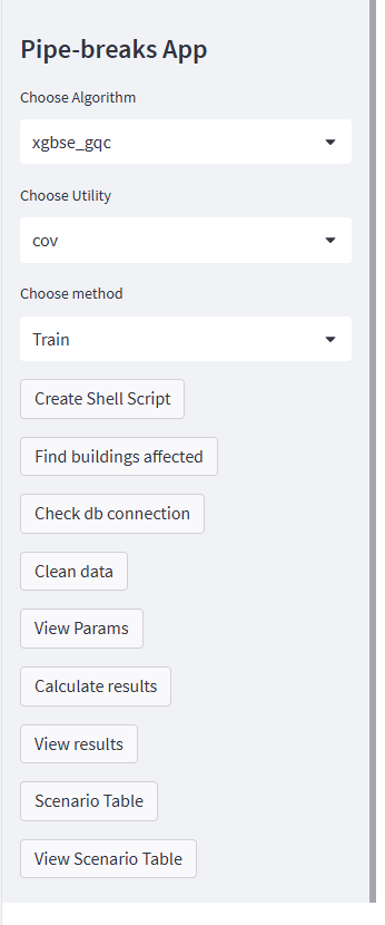
Algorithm Selection:

• Dropdown for selecting an algorithm (e.g., xgbse_gqc).

Utility Selection:

• Dropdown for selecting a utility (e.g., cov).

Method Selection:

• Dropdown for selecting a method (e.g., Train).

Buttons:

• Create Shell Script
• Find buildings affected
• Check db connection
• Clean data
• View Params
• Calculate results
• View results
• Scenario Table
• View Scenario Table

Inputs

User Inputs via Streamlit Sidebar:

• Algorithm selection
• Utility selection
• Method selection
• Button clicks for various actions (e.g., Create Shell Script, Find buildings affected, Check db connection, etc.)

Processes

Sidebar and Input Handling:

• User selects options and triggers actions through buttons.

Functions Executed Based on User Actions:

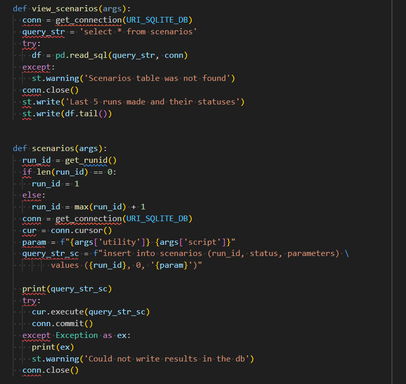
• create_shell_script(): Handles shell script creation.
• check(): Checks the database connection.
• dataset_for_surv_analysis(): Cleans and uploads data to the database.
• view_params(): Displays the parameters used to train the model.
• config(): Calculates results by configuring and running the specified algorithm.
• make_scatter(): Displays result graphs.
• scenarios(): Handles scenario table operations.
• view_scenarios(): Displays the scenario table.
• water_main(): Finds buildings affected by a water main break.
• wr(): Invoked if Transfer Learning is selected.

Outputs

Streamlit Interface:

• Various outputs based on user actions (e.g., success messages, parameter views, result views, etc.)
• Created shell script file.
• Database updates for scenarios.

LOE_COE Deepdive

app.py

1. Create Shell Script button Triggers create_shell_script() function.

   • Displays a form with inputs for nodes, GPUs, tasks, account, mail type, email, algorithm, and utility.
     • User provides input and presses the "Create SH file" button
       • Triggers make_sh(*args):
       • Collects form inputs.
       • Constructs SLURM directives and a Python command.
       • Saves the shell script file with the specified configuration.

2. User presses the "Find buildings affected" button:

   • Note : looks Like COE
   • Triggers water_main():
     • Collects the Asset ID.
     • Calls buildings_affected_by_watermain(asset_id).
       • Displays the list of buildings affected in the Streamlit interface.
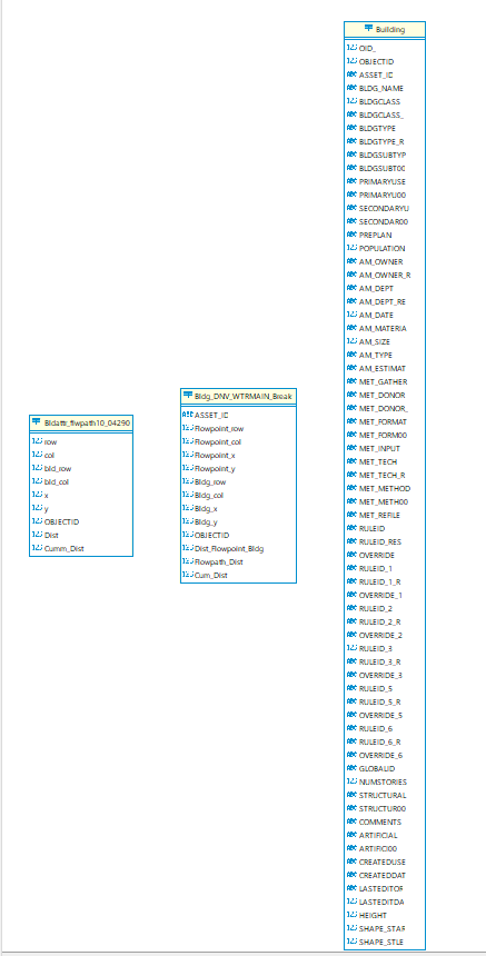
         • Connects to the buildings database i.e URI_BLGS_DB = "data/dnv_coe_buildings.db
         • Executes SQL queries to find buildings affected by the specified water main.
         • Merges the results of the queries into a single DataFrame.
         • Displays the affected buildings in the Streamlit interface.

3. User presses the "check" button:

   • Note : LOE
   • Triggers check():
   • Tests the connection to the database and displays the connection status
   • connects to URI_SQLITE_DB = "data/dnv_coe.db"(should rename to LOE)
   • Displays a success or failure message based on the connection status.

4. User presses the "check" button:

• Note : LOE

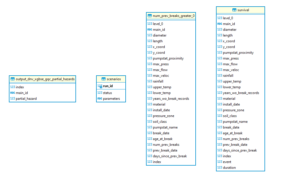
• Triggers dataset_for_surv_analysis()

  1. Database Check:

     • Connects to the SQLite database, connects to URI_SQLITE_DB = "data/dnv_coe.db"(should rename to LOE)
     • Checks if the survival table exists.

  2. Load Data:

     • If the survival table exists, loads data from the table.

  3. Process Data:

     • Cleans and processes the dataset, including handling missing values and calculating time-to-event.

  4. Merge Replacement Dates:

     • Loads replacement dates from a CSV file.
     • Merges the replacement dates with the main dataset.

  5. Calculate Duration:

     • Uses study period settings to calculate the duration for survival analysis.

  6. Save Data:

     • Writes the processed data to the survival table in the SQLite database.
     • Optionally saves the data to a CSV file if configured to do so.

5. User presses the "View Params" button:

• Note : LOE

• Triggers view_params()

  • Display Parameters:
  • Uses st.markdown() to display predefined model parameters in the Streamlit interface.

6. User presses the "Calculate Results" button:

- **Note** : doesn't work. LOE??


- Triggers `config(args)`
- **Process**:
    **Display Spinner**:
    - Displays a spinner in the Streamlit interface to indicate processing.

    **Load Configuration File**:
     - Loads the configuration file (`.toml`) for the specified utility.

7. User presses the "View Results" button:

   • Triggers make_scatter(args)
   • Generate Scatter Plots:
     • Uses the make_scatter() function to generate scatter plots based on the results.
   • Display Plots:
     • Displays the generated scatter plots in the Streamlit interface.

8. User presses the "Scenario Table" button:

   • Triggers scenarios(args)
   • Get Current Run ID:
   • Retrieves the current run ID from the database.
   • If no run ID exists, initializes it to 1. Otherwise, increments the maximum run ID by 1.

   Insert New Scenario Entry:

   • Inserts a new scenario entry into the scenarios table in the database with the new run ID, status (set to 0), and parameters.

9. User presses the "View Scenario Table" button:

- Triggers  `view_scenarios(args)`
- **Connect to Database**:
- Establishes a connection to the SQLite database.

- **Query Scenarios Table**:
- Executes a SQL query to fetch all entries from the `scenarios` table.

- **Display Results**:
- Displays the last five entries from the `scenarios` table in the    Streamlit interface.
- If the `scenarios` table is not found, displays a warning message.

ERD Diagrams

7/29/2024 :

Loe-Coe-app

• Tried running cov utility

Error Faced:

• Encountered a KeyError due to missing columns ('within_peat', 'grid_num', 'grid_num_breaks', 'upper_ph', 'lower_ph', 'upper_cond', 'lower_cond') in the dataset.

Solution:

• Added the following code to ensure the necessary columns are present in the dataset, initializing them with default values if they are missing

# Ensure all necessary columns are present
necessary_columns = ['within_peat', 'grid_num', 'grid_num_breaks', 'upper_ph', 'lower_ph', 'upper_cond', 'lower_cond']
for col in necessary_columns:
    if col not in data.columns:
        data[col] = 0  # or any default value

• This adjustment resolved the KeyError, allowing the program to run successfully.

7/30/2024 :

• prepared action items, pushed all my work and documented everything

7/31/2024 :

• edited the changes i made to cctv_ml py script added these changes t0 notebook 7 and had a succesfull run