Water_Quality_Analysis

Added a constituent using the Water_Quality_Analysis feature using HEC-RAS 6.5

Downloaded a model example from the HEC-RAS 6.5.

The spill model was mimicked by adding a constituent to the the example model which is under Documents-> Iniyaa-> hec ras resource-> Example_Projects_6_5-> Example_Projects-> Water Quality-> Nutrient Example

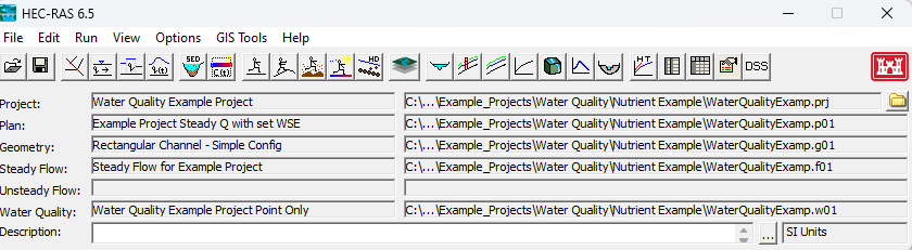
Go to Edit-> Water Quality Data to make changes to the model.

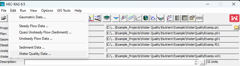
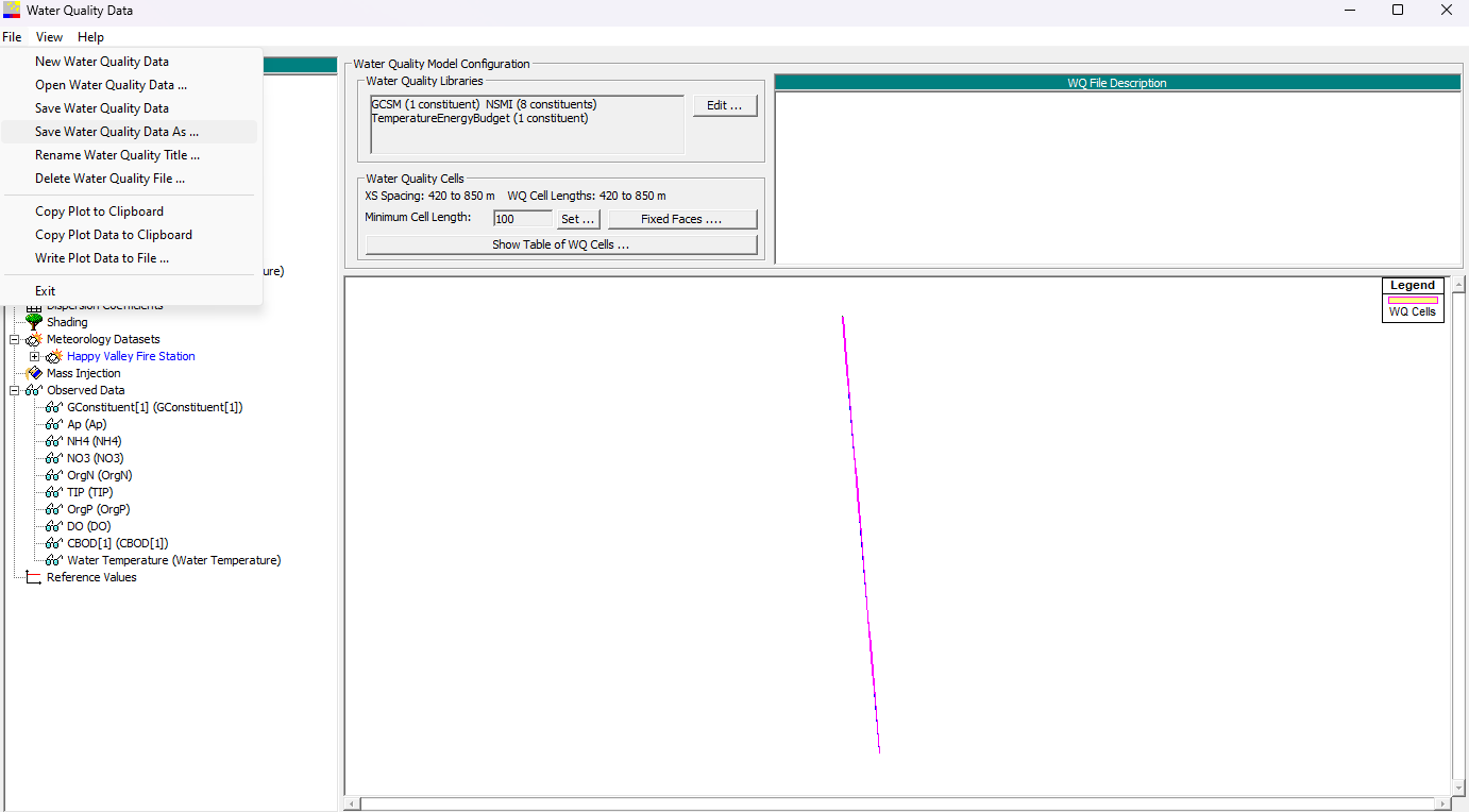
You ll have to create a new water quality analysis file first if you haven't created one before.

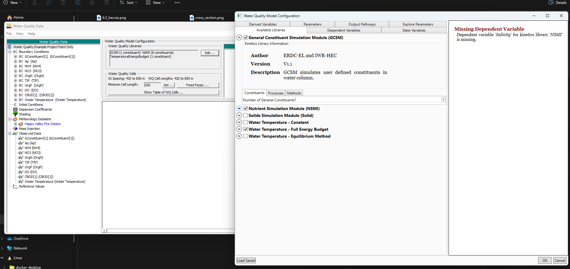
The GCSM simulates simple kinetics for up to ___ user-defined state variables. The number of constituents to be modeled is entered in the Water Quality Model Configuration Window as shown below. Once the number of constituents are entered, Added a constituent to the existing model- considering that constituent to be the oil spill. Select Edit from the Water Quality Model Configuration-> Select General Constituent Simulation Module (GCSM) and enter 1 as the number of constituents.

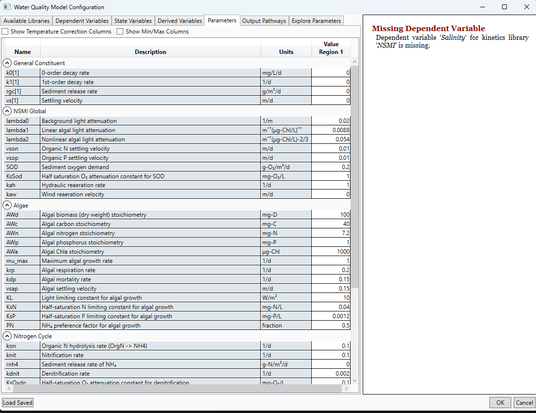
Parameters can be modified under the "Parameters" tab. All the parameters in the General constituent is set to zero for our spill model.

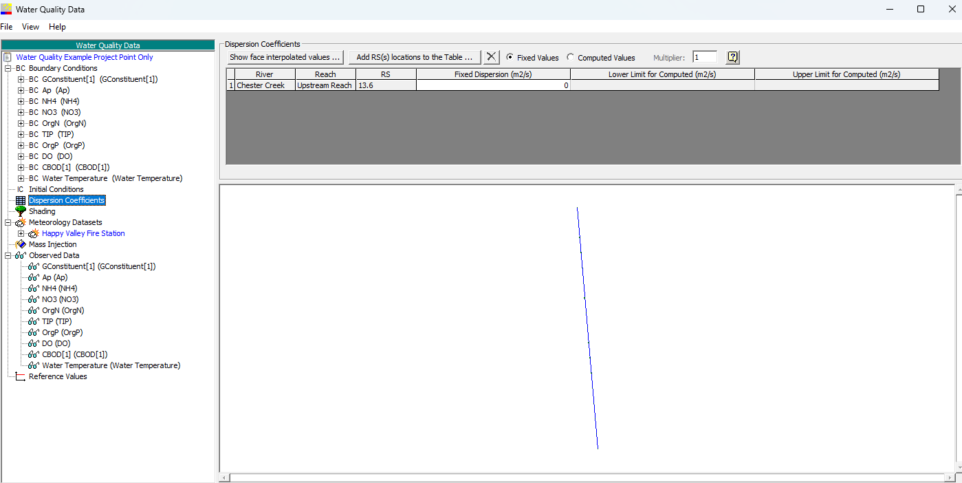
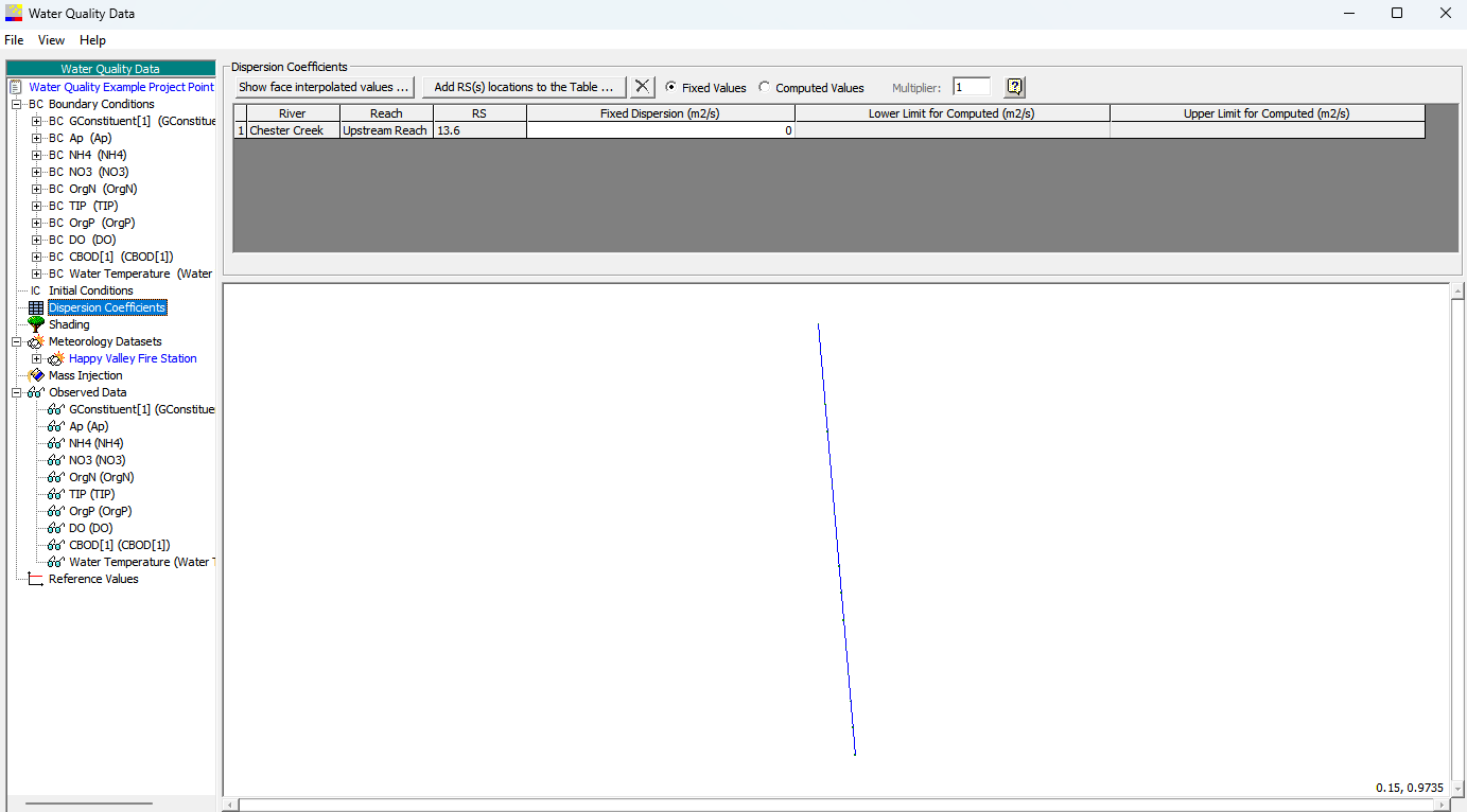
The dispersion coefficient can be modified in the Water Quality data editor as shown below. In our case, it is set to zero.

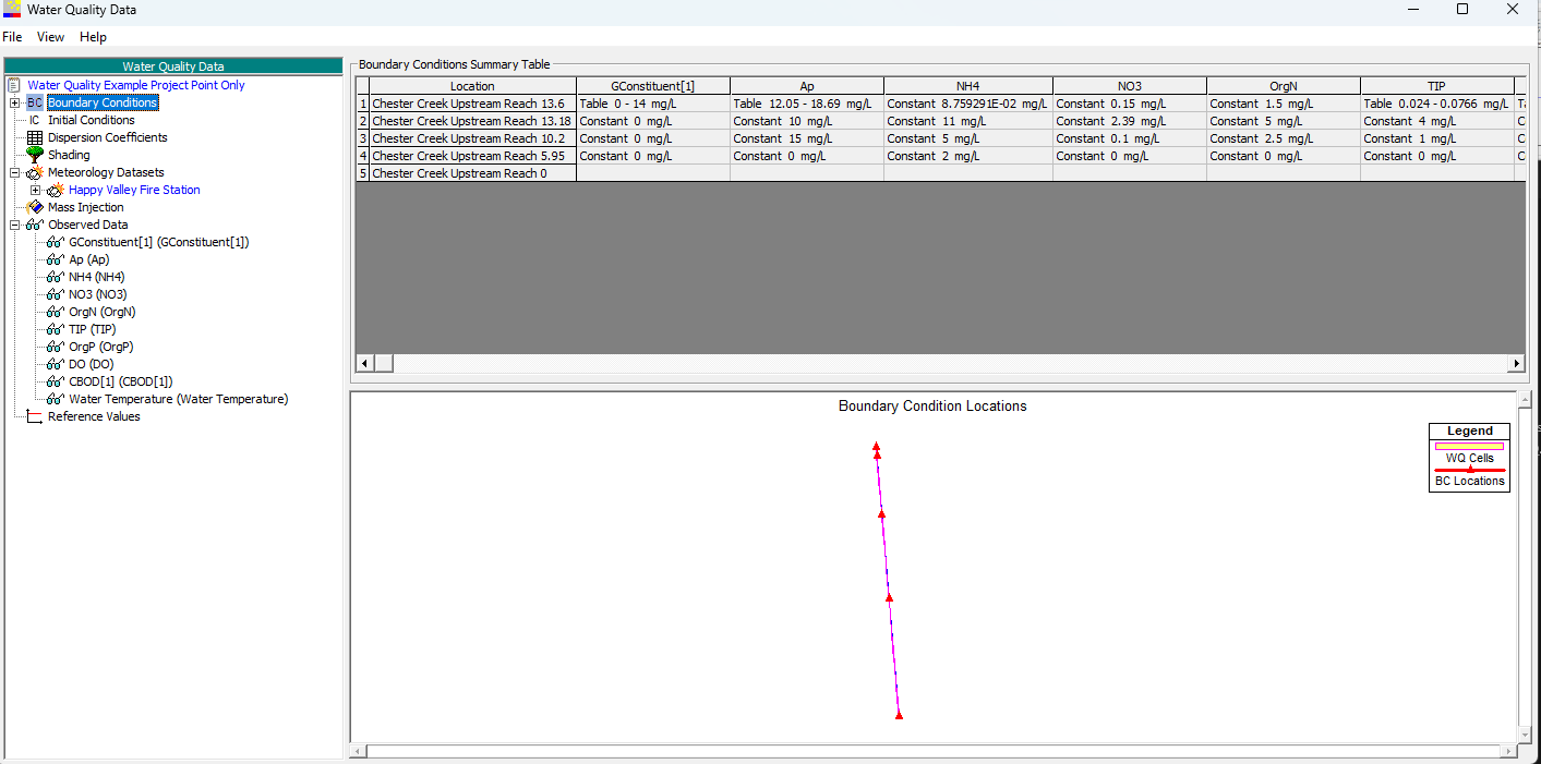
Now, we should set the boundary conditions.

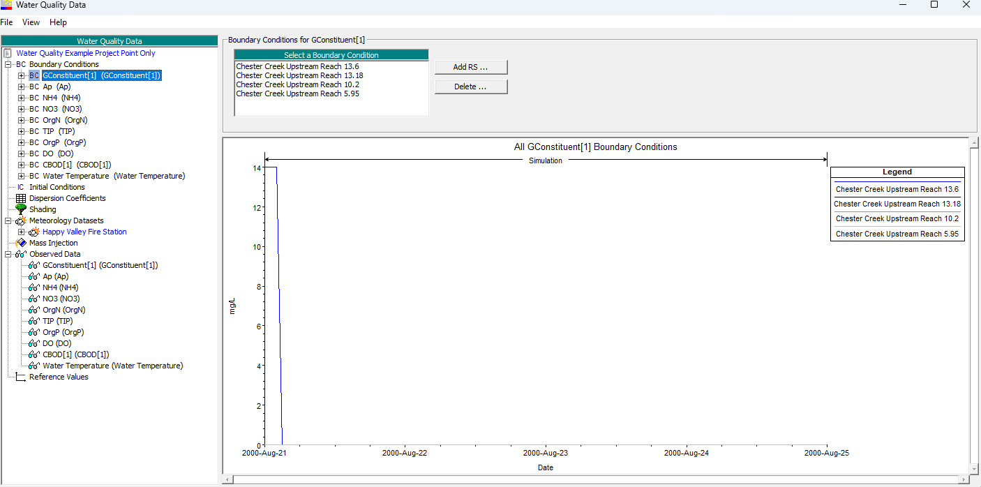
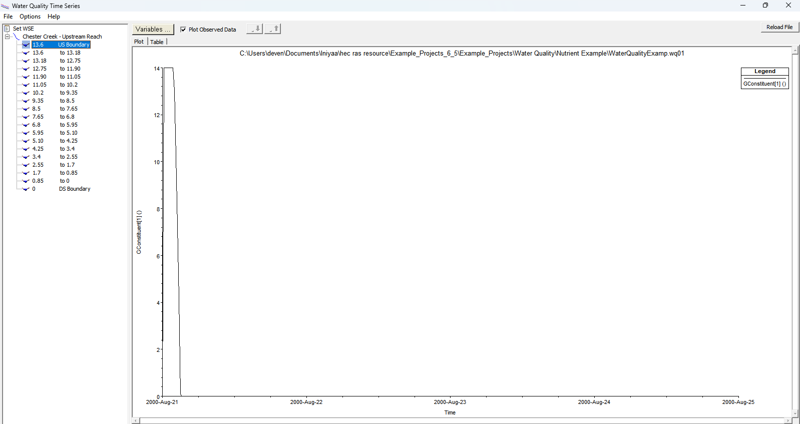
Considered a spill at the most upstream end of the cross section with concentration of 14 mg/L and the spill started from 0th hour to the 3rd hour.

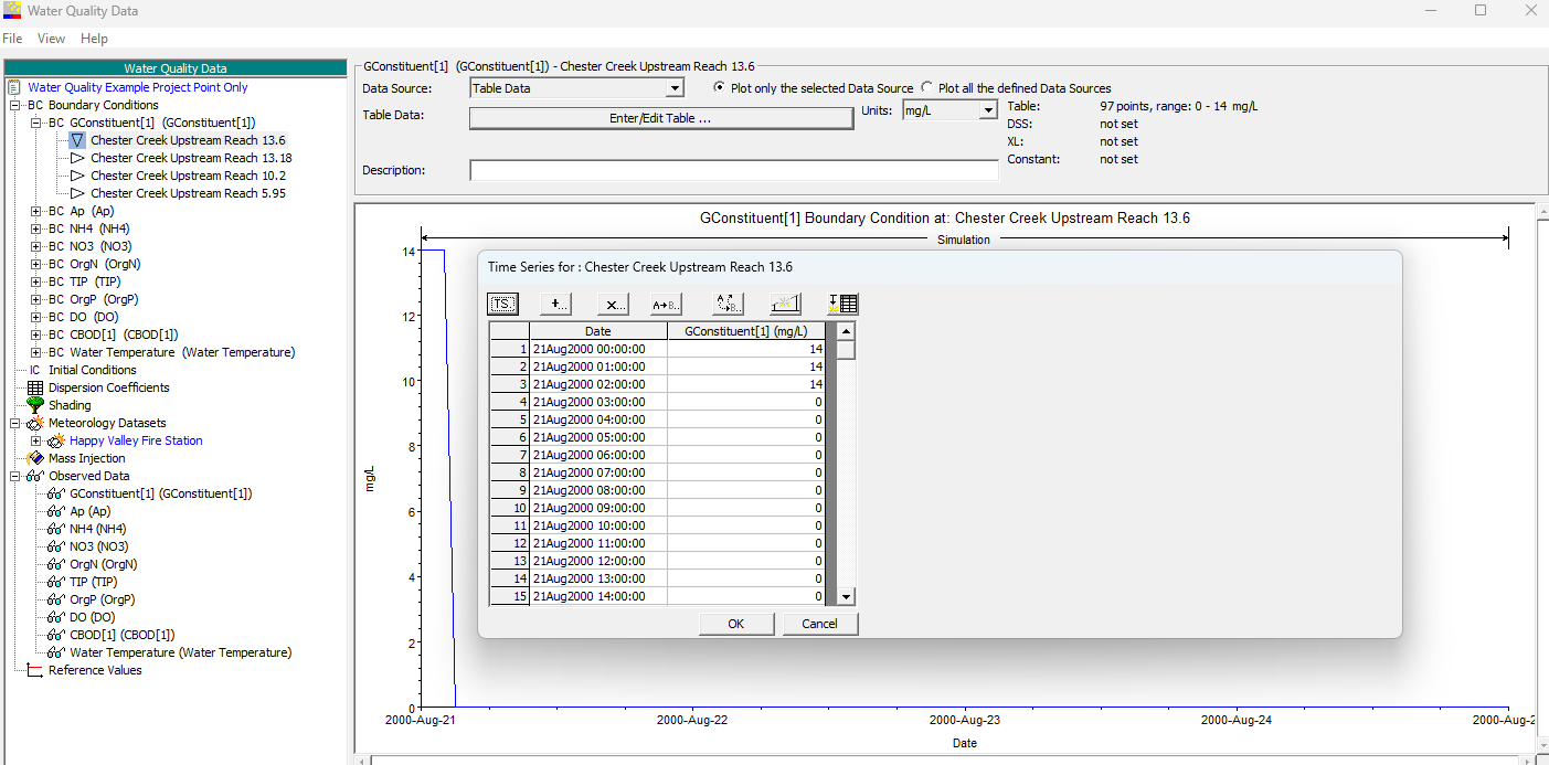
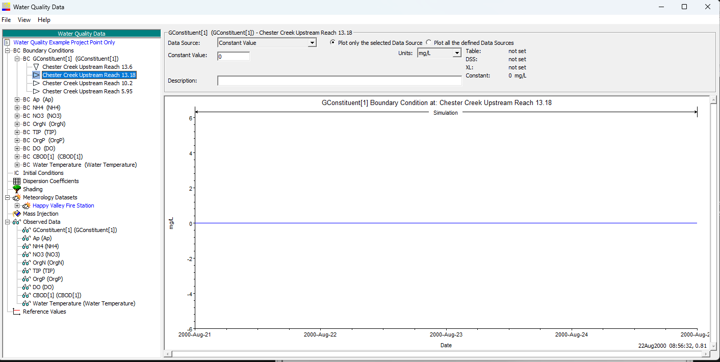
At the rest of the boundary conditions the concentration is set to a constant value=0 as we considered spill only happened at the upstream end of the cross section.

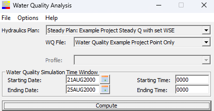
The model can be run now. Go to Run-> Water Quality Analysis...

To view the results after the run, you should go to View-> WQ Spatial plot or WQ Time series plot.

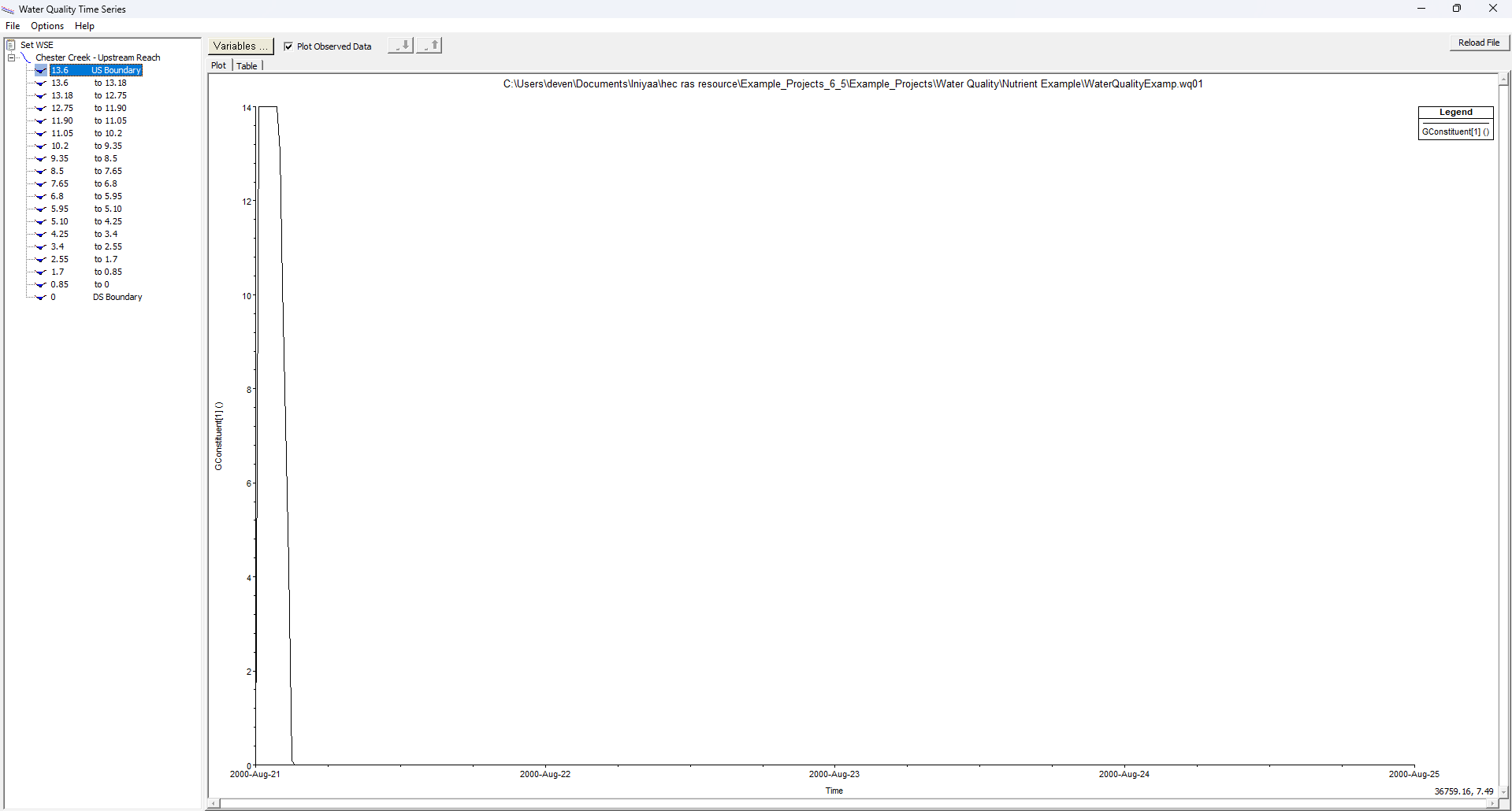
There's a decrease in the flow in 13.18 to 12.75 cross section from 14 mg/L to 8 mg/L. The reason could be due to additional lateral flow.

Other models

Water quality analysis was performed for Ohio river (East Palestine) and Russian River models. The model did not run.

Emails sent to HEC-RAS support

Iniyaa: "I was working with the water quality analysis and set the dispersion coefficient to zero. For the simulation, I used a square pulse for the spill simulation for 5 hours as the input. After running the simulation, I observed that the shape flattens out in the output, even though the dispersion coefficient was set to zero. This appears to be "numerical dispersion." Are there any plans to address this through new computational methods in future releases?"

Response from the HEC-RAS team:

"Hello Iniyaa,

After some digging into the condition of the RAS unsteady water quality, we have learned that the 6.4 and 6.5 version of the code are not operating. The last recommended version of RAS for use in unsteady water quality applications is version 6.3.1. Funding support for this module has been difficult to come by and it is not a high priority for the next release. We hope to get back to a functioning model but new water quality features will not be added in the near term.

I was able to access your Ohio model and take a look. This is a very complex hydraulic model for water quality use. Unsteady RAS water quality does not support storage areas, so the model would need to be reconfigured without storage areas for use in the water quality module at a minimum.

A link to the Water Quality User’s Manual is here for your reference. Please note the Technical Reference section which has a thorough discussion of how the model treats advection, dispersion, and diffusion: https://www.hec.usace.army.mil/confluence/rasdocs/raswqum

The advection diffusion transport used in HEC-RAS water quality is the QUICKEST ULTIMATE (Leanard). This approach essentially fits a quadratic around a face (XS) with one cell DS, one US and one for US (1 down and 2 upstream) and integrates the flow over the face for that time step. This is a second order approach, and the ULTIMATE part of the scheme is a limiter that reduces overestimates/oscillations from fitting a quadratic to a steep front. There is numerical dispersion in this approach, so one would not expect that setting the dispersion coefficient to zero would maintain a sharp front. There is a mixing in real water systems, so this is generally an acceptable consequence of the modeling approach. If you have calibration data for the mixing that occurs in your system you could calibrate the dispersion coefficients to the data and understand that the total dispersion in the model results would be the sum of the dispersion term with your coefficient and numerical dispersion from the advection portion of the solution. Using XS’s that are closer together and time steps that produce a courant = 1 will generally reduce the numerical dispersion.

The RAS team has limited ability to support non-USACE entities and we can’t offer much more help with this problem due to its non-trivial nature.

Regards, The RAS Team"